Multiple linear regression (MLR)

Categorical predictors + Assessment

Prof. Maria Tackett

Sep 12, 2024

Announcements

Lab 01 due on TODAY at 11:59pm
- Push work to GitHub repo
- Submit final PDF on Gradescope + mark pages for each question
HW 01 due Thursday, September 19 at 11:59pm
- Will be released after class
Team labs start on Monday

Homework

Homework will generally be split into two sections:

1️⃣ Conceptual exercises

The conceptual exercises are focused on explaining concepts and showing results mathematically. Show your work for each question.

You may write the answers and associated work for conceptual exercises by hand or type them in your Quarto document.

Homework

2️⃣ Applied exercises

The applied exercises are focused on applying the concepts to analyze data.

All work for the applied exercises must be typed in your Quarto document following a reproducible workflow.

Write all narrative using complete sentences and include informative axis labels / titles on visualizations.

Topics

Categorical predictors and interaction terms
Assess model fit using RSME and $R^2$
Compare models using $Adj. R^2$
Introduce LaTex

Computing setup

# load packages
library(tidyverse)
library(tidymodels)
library(openintro)
library(patchwork)
library(knitr)
library(kableExtra)
library(viridis) #adjust color palette

# set default theme and larger font size for ggplot2
ggplot2::theme_set(ggplot2::theme_minimal(base_size = 16))

Data: Peer-to-peer lender

Today’s data is a sample of 50 loans made through a peer-to-peer lending club. The data is in the loan50 data frame in the openintro R package.

# A tibble: 50 × 4
   annual_income_th debt_to_income verified_income interest_rate
              <dbl>          <dbl> <fct>                   <dbl>
 1             59           0.558  Not Verified            10.9 
 2             60           1.31   Not Verified             9.92
 3             75           1.06   Verified                26.3 
 4             75           0.574  Not Verified             9.92
 5            254           0.238  Not Verified             9.43
 6             67           1.08   Source Verified          9.92
 7             28.8         0.0997 Source Verified         17.1 
 8             80           0.351  Not Verified             6.08
 9             34           0.698  Not Verified             7.97
10             80           0.167  Source Verified         12.6 
# ℹ 40 more rows

Variables

Predictors:

annual_income_th: Annual income (in $1000s)
debt_to_income: Debt-to-income ratio, i.e. the percentage of a borrower’s total debt divided by their total income
verified_income: Whether borrower’s income source and amount have been verified (Not Verified, Source Verified, Verified)

Response: interest_rate: Interest rate for the loan

Response vs. predictors

Goal: Use these predictors in a single model to understand variability in interest rate.

Model fit in R

int_fit <- lm(interest_rate ~ debt_to_income + verified_income  + annual_income_th,
              data = loan50)

tidy(int_fit) |>
  kable(digits = 3)

term	estimate	std.error	statistic	p.value
(Intercept)	10.726	1.507	7.116	0.000
debt_to_income	0.671	0.676	0.993	0.326
verified_incomeSource Verified	2.211	1.399	1.581	0.121
verified_incomeVerified	6.880	1.801	3.820	0.000
annual_income_th	-0.021	0.011	-1.804	0.078

Categorical predictors

Matrix form of multiple linear regression

\[ \underbrace{ \begin{bmatrix} y_1 \\ \vdots \\ y_n \end{bmatrix} }_ {\mathbf{y}} \hspace{3mm} = \hspace{3mm} \underbrace{ \begin{bmatrix} 1 &x_{11} & \dots & x_{1p}\\ \vdots & \vdots &\ddots & \vdots \\ 1 & x_{n1} & \dots &x_{np} \end{bmatrix} }_{\mathbf{X}} \hspace{2mm} \underbrace{ \begin{bmatrix} \beta_0 \\ \beta_1 \\ \vdots \\ \beta_p \end{bmatrix} }_{\boldsymbol{\beta}} \hspace{3mm} + \hspace{3mm} \underbrace{ \begin{bmatrix} \epsilon_1 \\ \vdots\\ \epsilon_n \end{bmatrix} }_\boldsymbol{\epsilon} \]

How might we include a categorical predictor with $k$ levels in the design matrix, $\mathbf{X}$ ?

Indicator variables

Suppose we want to predict the amount of sleep a Duke student gets based on whether they are in Pratt (Pratt Yes/ No are the only two options). Consider the model

\[ Sleep_i = \beta_0 + \beta_1\mathbf{1}(Pratt_i = \texttt{Yes}) + \beta_2\mathbf{1}(Pratt_i = \texttt{No}) \]

Write out the design matrix for this hypothesized linear model.
Demonstrate that the design matrix is not of full column rank (that is, affirmatively provide one of the columns in terms of the others).
Use this intuition to explain why when we include categorical predictors, we cannot include both indicators for every level of the variable and an intercept.

Indicator variables

Suppose there is a categorical variable with $k$ levels
We can make $k$ indicator variables from the data - one indicator for each level
An indicator (dummy) variable takes values 1 or 0
- 1 if the observation belongs to that level
- 0 if the observation does not belong to that level

Indicator variables for `verified_income`

loan50 <- loan50 |>
  mutate(
    not_verified = if_else(verified_income == "Not Verified", 1, 0),
    source_verified = if_else(verified_income == "Source Verified", 1, 0),
    verified = if_else(verified_income == "Verified", 1, 0)
  )

# A tibble: 3 × 4
  verified_income not_verified source_verified verified
  <fct>                  <dbl>           <dbl>    <dbl>
1 Not Verified               1               0        0
2 Verified                   0               0        1
3 Source Verified            0               1        0

Indicator variables in the model

We will use $k-1$ of the indicator variables in the model.
The baseline is the category that doesn’t have a term in the model.
The coefficients of the indicator variables in the model are interpreted as the expected change in the response compared to the baseline, holding all other variables constant.

loan50 |>
  select(verified_income, source_verified, verified) |>
  slice(1, 3, 6)

# A tibble: 3 × 3
  verified_income source_verified verified
  <fct>                     <dbl>    <dbl>
1 Not Verified                  0        0
2 Verified                      0        1
3 Source Verified               1        0

Take a look at the design matrix in AE 02

Interpreting `verified_income`

term	estimate	std.error	statistic	p.value	conf.low	conf.high
(Intercept)	10.726	1.507	7.116	0.000	7.690	13.762
debt_to_income	0.671	0.676	0.993	0.326	-0.690	2.033
verified_incomeSource Verified	2.211	1.399	1.581	0.121	-0.606	5.028
verified_incomeVerified	6.880	1.801	3.820	0.000	3.253	10.508
annual_income_th	-0.021	0.011	-1.804	0.078	-0.043	0.002

The baseline level is Not verified.
People with source verified income are expected to take a loan with an interest rate that is 2.211% higher, on average, than the rate on loans to those whose income is not verified, holding all else constant.

What is the expected interest rate for someone whose income is Verified, who has a debt-to-income ratio of 0 and annual income of $0?

Interaction terms

Sometimes the relationship between a predictor variable and the response depends on the value of another predictor variable.
This is an interaction effect.
To account for this, we can include interaction terms in the model.

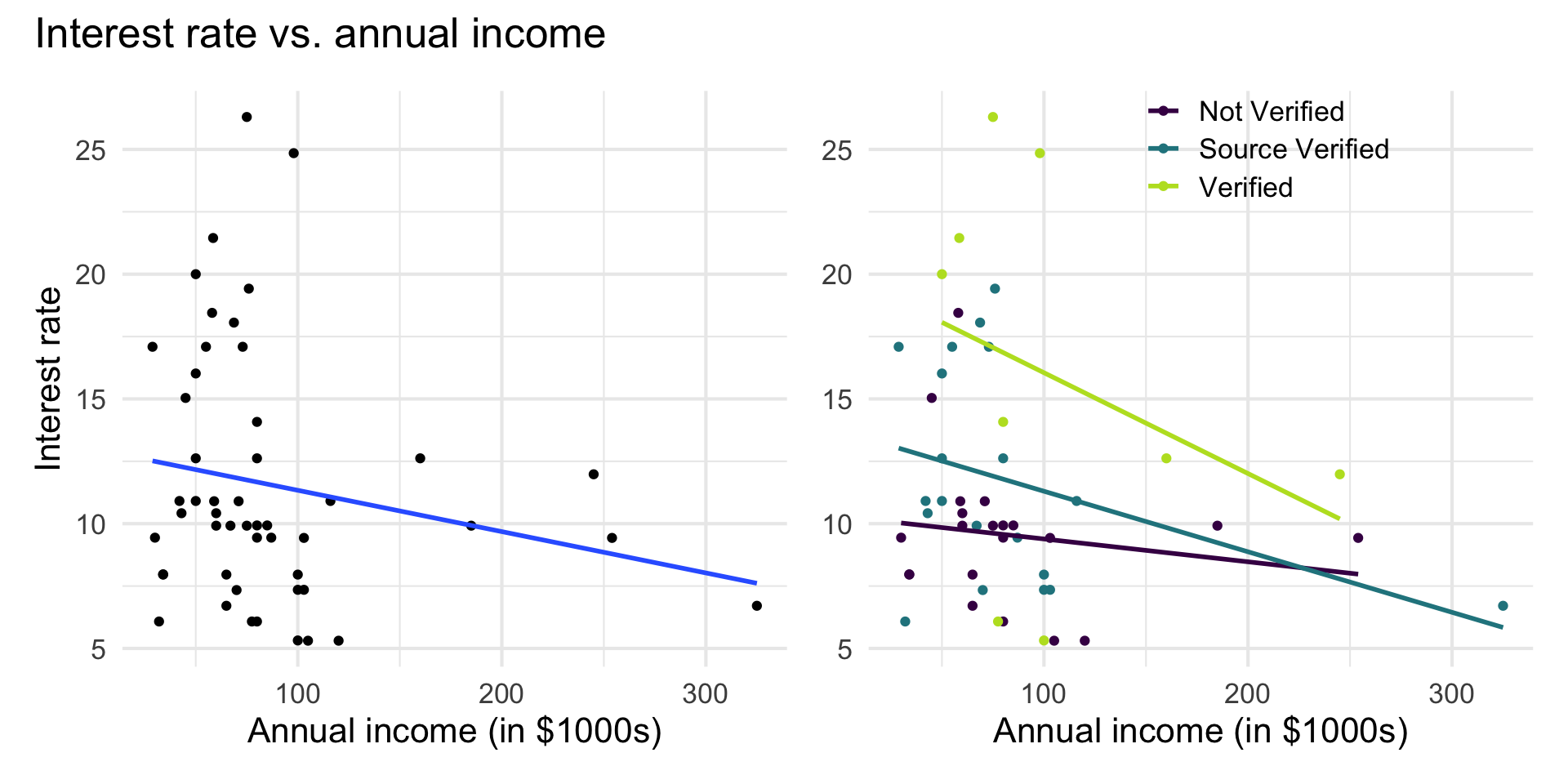
Interest rate vs. annual income

The lines are not parallel indicating there is a potential interaction effect. The slope of annual income differs based on the income verification.

Application exercise

📋 https://sta221-fa24.netlify.app/ae/ae-02-mlr

Interaction term in model

int_fit_2 <- lm(interest_rate ~ debt_to_income + verified_income + annual_income_th + verified_income * annual_income_th,
      data = loan50)

term	estimate	std.error	statistic	p.value
(Intercept)	9.560	2.034	4.700	0.000
debt_to_income	0.691	0.685	1.009	0.319
verified_incomeSource Verified	3.577	2.539	1.409	0.166
verified_incomeVerified	9.923	3.654	2.716	0.009
annual_income_th	-0.007	0.020	-0.341	0.735
verified_incomeSource Verified:annual_income_th	-0.016	0.026	-0.643	0.523
verified_incomeVerified:annual_income_th	-0.032	0.033	-0.979	0.333

Interpreting interaction terms

What the interaction means: The effect of annual income on the interest rate differs by -0.016 when the income is source verified compared to when it is not verified, holding all else constant.
Interpreting annual_income for source verified: If the income is source verified, we expect the interest rate to decrease by 0.023% (-0.007 + -0.016) for each additional thousand dollars in annual income, holding all else constant.

Model assessment and comparison

RMSE & $R^2$

Root mean square error, RMSE: A measure of the average error (average difference between observed and predicted values of the outcome)
R-squared, $R^2$ : Percentage of variability in the outcome explained by the regression model

Comparing models

When comparing models, do we prefer the model with the lower or higher RMSE?
Though we use $R^2$ to assess the model fit, it is generally unreliable for comparing models with different number of predictors. Why?
- $R^2$ will stay the same or increase as we add more variables to the model . Let’s show why this is true.
- If we only use $R^2$ to choose a best fit model, we will be prone to choose the model with the most predictor variables.

Adjusted $R^2$

Adjusted $R^2$: measure that includes a penalty for unnecessary predictor variables
Similar to $R^2$, it is a measure of the amount of variation in the response that is explained by the regression model

$R^2$ and Adjusted $R^2$

\[R^2 = \frac{SSM}{SST} = 1 - \frac{SSR}{SST}\]

\[R^2_{adj} = 1 - \frac{SSR/(n-p-1)}{SST/(n-1)}\]

where

$n$ is the number of observations used to fit the model
$p$ is the number of terms (not including the intercept) in the model

Using $R^2$ and Adjusted $R^2$

Adjusted $R^2$ can be used as a quick assessment to compare the fit of multiple models; however, it should not be the only assessment!
Use $R^2$ when describing the relationship between the response and predictor variables

📋 https://sta221-fa24.netlify.app/ae/ae-02-mlr

LaTex

Latex in this class

For this class you will need to be able to…

Properly write mathematical symbols, e.g., $\beta_1$ not B1, $R^2$ not R2
Write basic regression equations, e.g., $\hat{y} = \beta_0 + \beta_1x_1 + \beta_2x_2$
Write matrix equations: $\mathbf{y} = \mathbf{X}\boldsymbol{\beta} + \boldsymbol{\epsilon}$
Write hypotheses (we’ll start this next week), e.g., $H_0: \beta = 0$

You are welcome to but not required to write math proofs using LaTex.

Application exercise

📋 https://sta221-fa24.netlify.app/ae/ae-02-mlr

Recap

Interpreted categorical predictors and interaction terms
Assessed model fit using RSME and $R^2$
Compared models using $Adj. R^2$
Introduced LaTex

Next class

Geometric interpretation
Inference for regression
See Sep 17 prepare

Multiple linear regression (MLR)

Announcements

Homework

Homework

Topics

Computing setup

Data: Peer-to-peer lender

Variables

Response vs. predictors

Model fit in R

Categorical predictors

Matrix form of multiple linear regression

Indicator variables

Indicator variables

Indicator variables for `verified_income`

Indicator variables in the model

Interpreting `verified_income`

Interaction terms

Interaction terms

Interest rate vs. annual income

Application exercise

Interaction term in model

Interpreting interaction terms

Model assessment and comparison

RMSE & \(R^2\)

Comparing models

Adjusted \(R^2\)

\(R^2\) and Adjusted \(R^2\)

Using \(R^2\) and Adjusted \(R^2\)

LaTex

Latex in this class

Application exercise

Recap

Next class

Multiple linear regression (MLR)

Announcements

Homework

Homework

Topics

Computing setup

Data: Peer-to-peer lender

Variables

Response vs. predictors

Model fit in R

Categorical predictors

Matrix form of multiple linear regression

Indicator variables

Indicator variables

Indicator variables for verified_income

Indicator variables in the model

Interpreting verified_income

Interaction terms

Interaction terms

Interest rate vs. annual income

Application exercise

Interaction term in model

Interpreting interaction terms

Model assessment and comparison

RMSE & \(R^2\)

Comparing models

Adjusted \(R^2\)

\(R^2\) and Adjusted \(R^2\)

Using \(R^2\) and Adjusted \(R^2\)

LaTex

Latex in this class

Application exercise

Recap

Next class

Indicator variables for `verified_income`

Interpreting `verified_income`