Inference for regression
cont’d
Sep 24, 2024
Announcements
Project
Research questions due Thursday at 11:59pm
Proposal due Thursday, October 3 at 11:59pm
Lab 03 due Thursday, October 3 at 11:59pm
Statistics experience due Tue, Nov 26 at 11:59pm
Topics
Understand statistical inference in the context of regression
Describe the assumptions for regression
Understand connection between distribution of residuals and inferential procedures
Conduct inference on a single coefficient
Conduct inference on the overall regression model
Computing setup
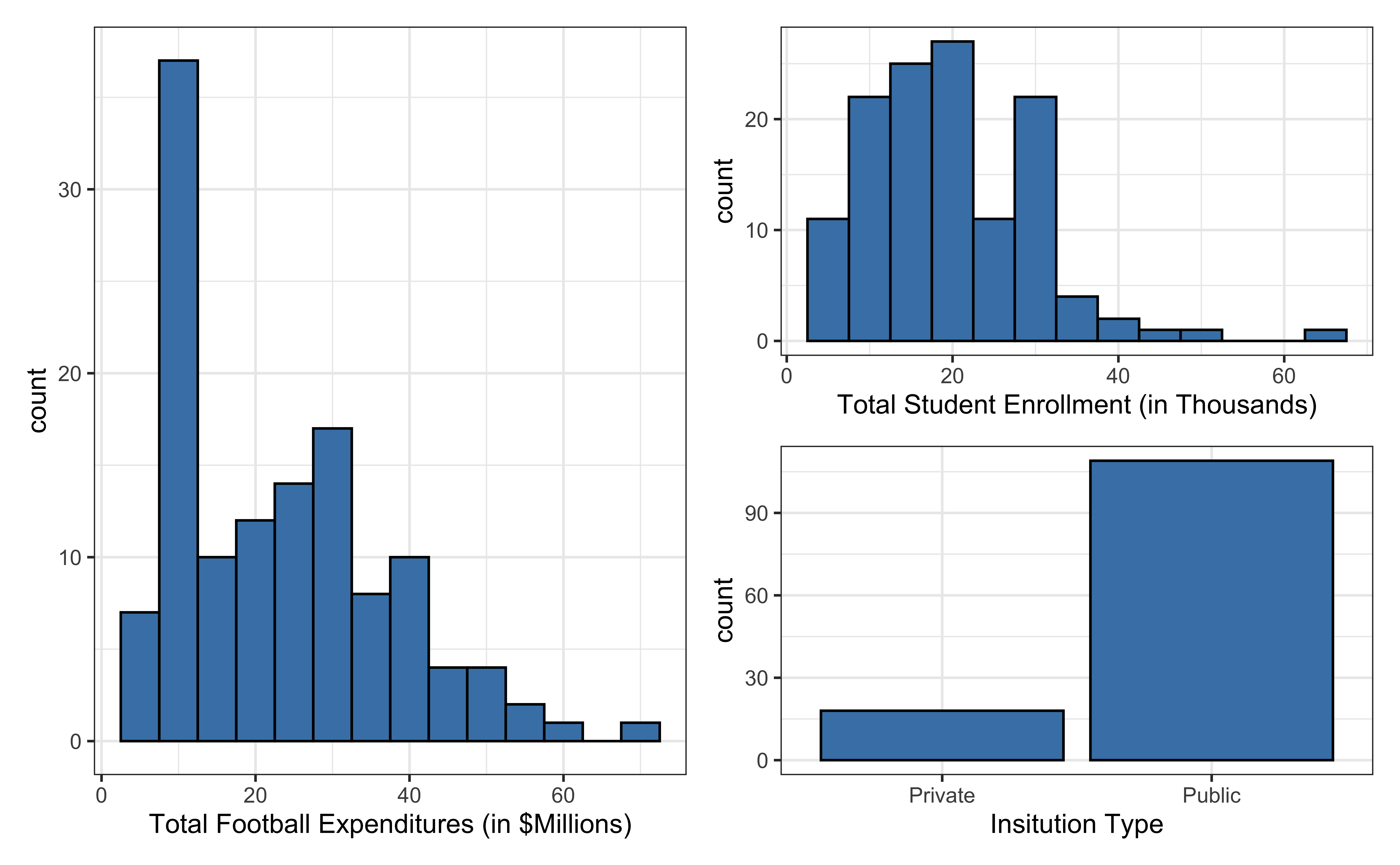
Data: NCAA Football expenditures
Today’s data come from Equity in Athletics Data Analysis and includes information about sports expenditures and revenues for colleges and universities in the United States. This data set was featured in a March 2022 Tidy Tuesday.
We will focus on the 2019 - 2020 season expenditures on football for institutions in the NCAA - Division 1 FBS. The variables are :
total_exp_m: Total expenditures on football in the 2019 - 2020 academic year (in millions USD)enrollment_th: Total student enrollment in the 2019 - 2020 academic year (in thousands)type: institution type (Public or Private)
Univariate EDA
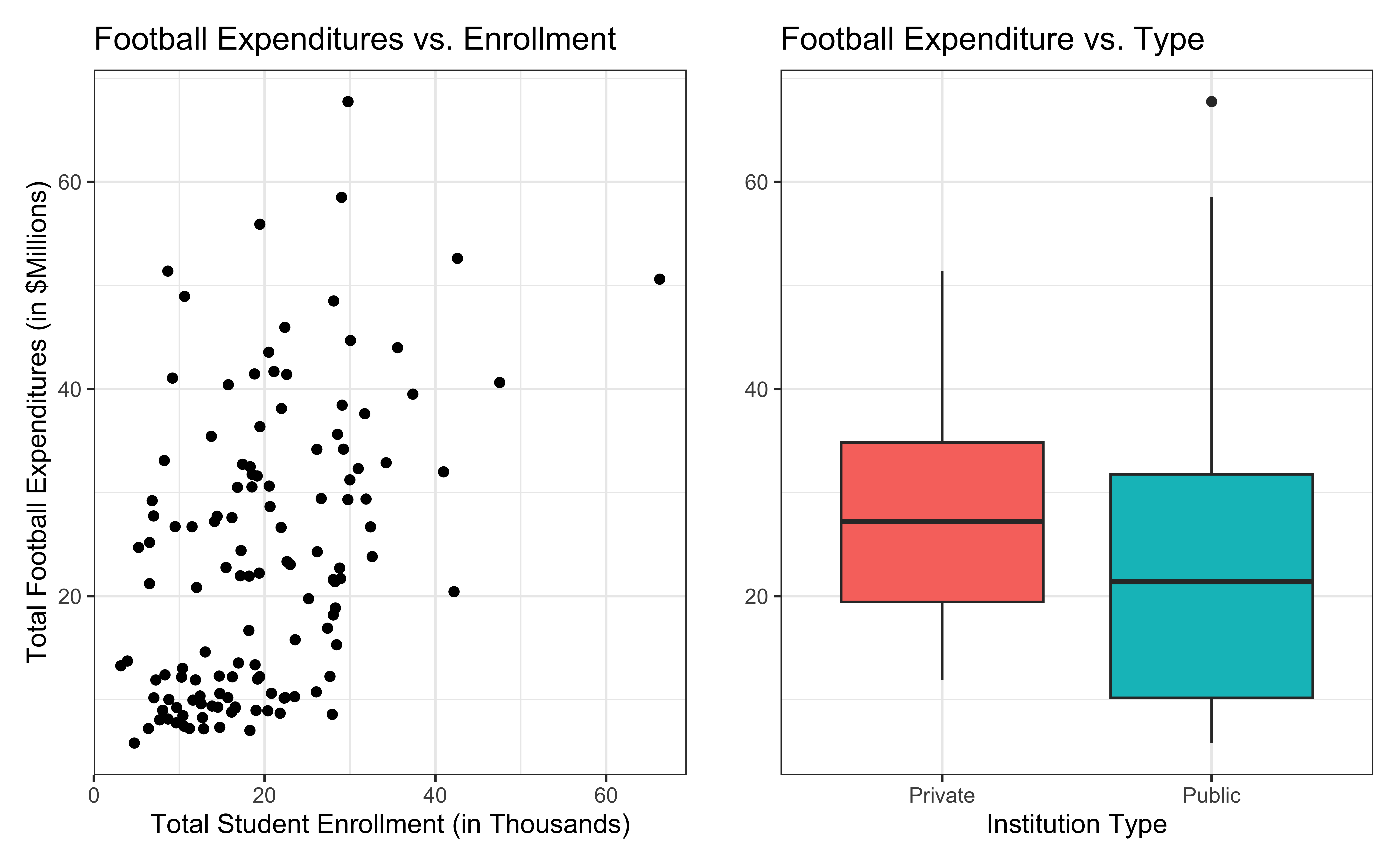
Bivariate EDA
Regression model
exp_fit <- lm(total_exp_m ~ enrollment_th + type, data = football)
tidy(exp_fit) |>
kable(digits = 3)| term | estimate | std.error | statistic | p.value |
|---|---|---|---|---|
| (Intercept) | 19.332 | 2.984 | 6.478 | 0 |
| enrollment_th | 0.780 | 0.110 | 7.074 | 0 |
| typePublic | -13.226 | 3.153 | -4.195 | 0 |
For every additional 1,000 students, we expect the institution’s total expenditures on football to increase by $780,000, on average, holding institution type constant.
Inference for regression
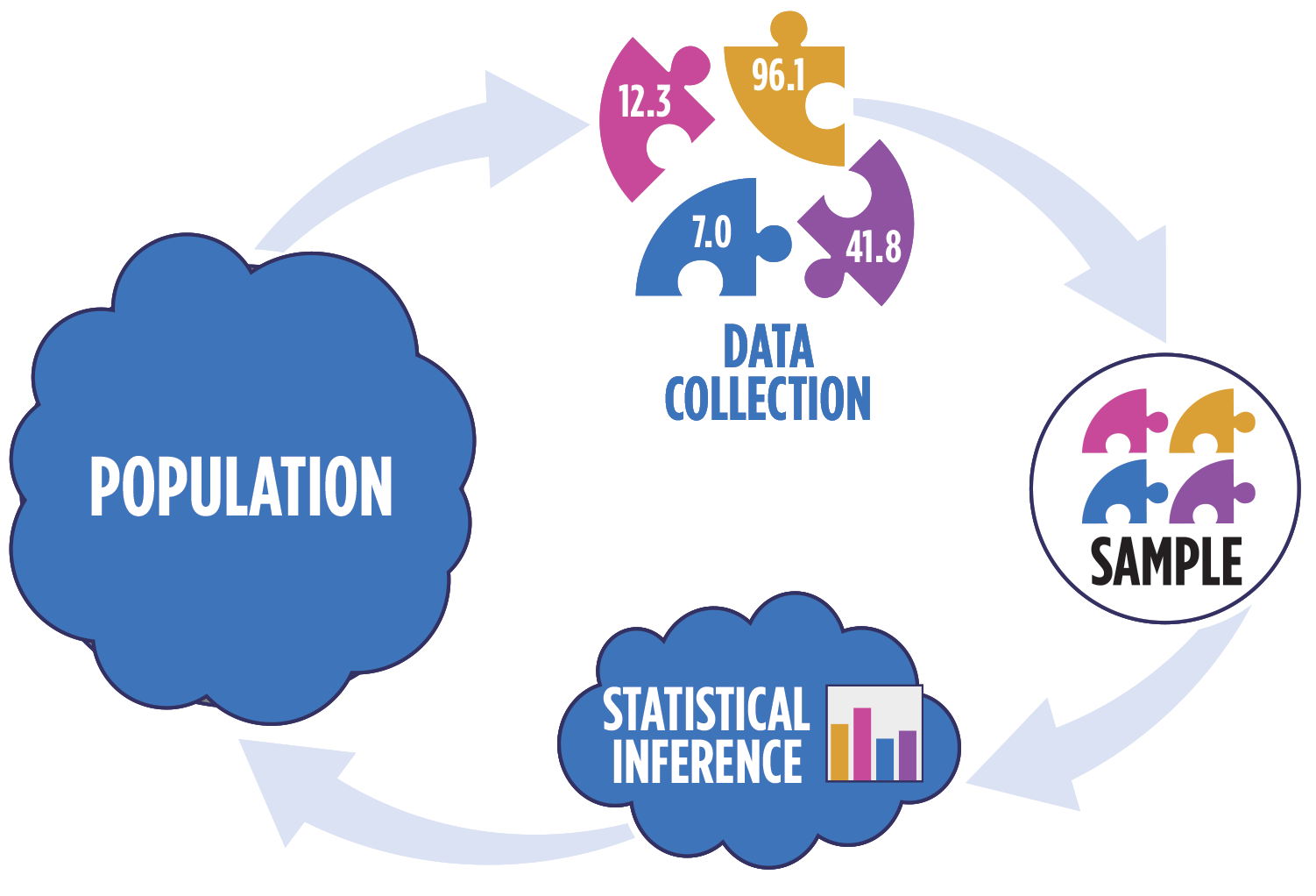
Statistical inference
Statistical inference provides methods and tools so we can use the single observed sample to make valid statements (inferences) about the population it comes from
For our inferences to be valid, the sample should be representative (ideally random) of the population we’re interested in
Inference for linear regression
Inference based on ANOVA
Hypothesis test for the statistical significance of the overall regression model
Hypothesis test for a subset of coefficients
Inference for a single coefficient \(\beta_j\)
Hypothesis test for a coefficient \(\beta_j\)
Confidence interval for a coefficient \(\beta_j\)
Linear regression model
\[ \begin{aligned} \mathbf{y} &= Model + Error \\[5pt] &= f(\mathbf{X}) + \boldsymbol{\epsilon} \\[5pt] &= E(\mathbf{y}|\mathbf{X}) + \mathbf{\epsilon} \\[5pt] &= \mathbf{X}\boldsymbol{\beta} + \mathbf{\epsilon} \end{aligned} \]
We have discussed multiple ways to find the least squares estimates of \(\boldsymbol{\beta} = \begin{bmatrix}\beta_0 \\\beta_1\end{bmatrix}\)
- None of these approaches depend on the distribution of \(\boldsymbol{\epsilon}\)
Now we will use statistical inference to draw conclusions about \(\boldsymbol{\beta}\) that depend on particular assumptions about the distribution of \(\boldsymbol{\epsilon}\)
Linear regression model
\[ \mathbf{y}|\mathbf{X} \sim N(\mathbf{X}\boldsymbol{\beta}, \sigma_\epsilon^2\mathbf{I}) \]
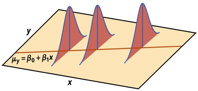
Image source: Introduction to the Practice of Statistics (5th ed)
Expected value of \(\mathbf{y}\)
Let \(\mathbf{b} = \begin{bmatrix}b_1 \\ \vdots \\b_p\end{bmatrix}\) be a \(p \times 1\) vector of random variables.
Then \(E(\mathbf{b}) = E\begin{bmatrix}b_1 \\ \vdots \\ b_p\end{bmatrix} = \begin{bmatrix}E(b_1) \\ \vdots \\ E(b_p)\end{bmatrix}\)
Use this to find \(E(\mathbf{y}|\mathbf{X})\).
Variance
Let \(\mathbf{b} = \begin{bmatrix}b_1 \\ \vdots \\b_p\end{bmatrix}\) be a \(p \times 1\) vector of independent random variables.
Then \(Var(\mathbf{b}) = \begin{bmatrix}Var(b_1) & 0 & \dots & 0 \\ 0 & Var(b_2) & \dots & 0 \\ \vdots & \vdots & \dots & \cdot \\ 0 & 0 & \dots & Var(b_p)\end{bmatrix}\)
Use this to find \(Var(\mathbf{y}|\mathbf{X})\).
Assumptions of regression
\[ \mathbf{y}|\mathbf{X} \sim N(\mathbf{X}\boldsymbol{\beta}, \sigma_\epsilon^2\mathbf{I}) \]
- Linearity: There is a linear relationship between the response and predictor variables.
- Constant Variance: The variability about the least squares line is generally constant.
- Normality: The distribution of the residuals is approximately normal.
- Independence: The residuals are independent from one another.
Estimating \(\sigma^2_{\epsilon}\)
Once we fit the model, we can use the residuals to estimate \(\sigma_{\epsilon}^2\)
\(\hat{\sigma}^2_{\epsilon}\) is needed for hypothesis testing and constructing confidence intervals for regression
\[ \hat{\sigma}^2_\epsilon = \frac{\sum_\limits{i=1}^n(y_i - \hat{y}_i)^2}{n-p-1} = \frac{\sum_\limits{i=1}^ne_i^2}{n - p - 1} = \frac{SSR}{n - p - 1} \]
- The regression standard error \(\hat{\sigma}_{\epsilon}\) is a measure of the average distance between the observations and regression line
\[ \hat{\sigma}_\epsilon = \sqrt{\frac{SSR}{n - p - 1}} \]
Inference for a single coefficient
Inference for \(\beta_j\)
We often want to conduct inference on individual model coefficients
Hypothesis test: Is there a linear relationship between the response and \(x_j\)?
Confidence interval: What is a plausible range of values \(\beta_j\) can take?
But first we need to understand the distribution of \(\hat{\beta}_j\)
Sampling distribution of \(\hat{\beta}_j\)
\[ \hat{\boldsymbol{\beta}} \sim N(\boldsymbol{\beta}, \sigma^2_\epsilon(\mathbf{X}^T\mathbf{X})^{-1}) \]
Let \(\mathbf{C} = (\mathbf{X}^T\mathbf{X})^{-1}\). Then, for each coefficient \(\hat{\beta}_j\),
\(E(\hat{\beta}_j) = \boldsymbol{\beta}_j\), the \(j^{th}\) element of \(\boldsymbol{\beta}\)
\(Var(\hat{\beta}_j) = \sigma^2_{\epsilon}C_{jj}\)
\(Cov(\hat{\beta}_i, \hat{\beta}_j) = \sigma^2_{\epsilon}C_{ij}\)
Hypothesis test for \(\beta_j\)
Steps for a hypothesis test
- State the null and alternative hypotheses.
- Calculate a test statistic.
- Calculate the p-value.
- State the conclusion.
Hypothesis test for \(\beta_j\): Hypotheses
We will generally test the hypotheses:
Null Hypothesis: \(H_0: \beta_j = 0\)
- There is no linear relationship between \(\beta_j\) and \(y\) after accounting for the other variables in the model
Alternative hypothesis: \(H_a: \beta_j \neq 0\)
- There is a linear relationship between \(\beta_j\) and \(y\) after accounting for the other variables in the model
Hypothesis test for \(\beta_j\): Test statistic
Test statistic: Number of standard errors the estimate is away from the null hypothesized value
\[ \text{Test Statstic} = \frac{\text{Estimate - Null}}{\text{Standard error}} \\ \]
\[T = \frac{\hat{\beta}_j - 0}{SE(\hat{\beta}_j)} ~ = ~\frac{\hat{\beta}_j - 0}{\sqrt{\hat{\sigma}^2_\epsilon C_{jj}}} ~\sim ~ t_{n-p-1} \]
Hypothesis test for \(\beta_j\): P-value
The p-value is the probability of observing a test statistic at least as extreme (in the direction of the alternative hypothesis) from the null value as the one observed
\[ p-value = P(|t| > |\text{test statistic}|), \]
calculated from a \(t\) distribution with \(n- p - 1\) degrees of freedom
Understanding the p-value
| Magnitude of p-value | Interpretation |
|---|---|
| p-value < 0.01 | strong evidence against \(H_0\) |
| 0.01 < p-value < 0.05 | moderate evidence against \(H_0\) |
| 0.05 < p-value < 0.1 | weak evidence against \(H_0\) |
| p-value > 0.1 | effectively no evidence against \(H_0\) |
These are general guidelines. The strength of evidence depends on the context of the problem.
Hypothesis test for \(\beta_j\): Conclusion
There are two parts to the conclusion
Make a conclusion by comparing the p-value to a predetermined decision-making threshold called the significance level ( \(\alpha\) level)
If \(\text{p-value} < \alpha\): Reject \(H_0\)
If \(\text{p-value} \geq \alpha\): Fail to reject \(H_0\)
State the conclusion in the context of the data
Application exercise
Confidence interval for \(\beta_j\)
Confidence interval for \(\beta_j\)
A plausible range of values for a population parameter is called a confidence interval
Using only a single point estimate is like fishing in a murky lake with a spear, and using a confidence interval is like fishing with a net
We can throw a spear where we saw a fish but we will probably miss, if we toss a net in that area, we have a good chance of catching the fish
Similarly, if we report a point estimate, we probably will not hit the exact population parameter, but if we report a range of plausible values we have a good shot at capturing the parameter
What “confidence” means
We will construct \(C\%\) confidence intervals.
- The confidence level impacts the width of the interval
- “Confident” means if we were to take repeated samples of the same size as our data, fit regression lines using the same predictors, and calculate \(C\%\) CIs for the coefficient of \(x_j\), then \(C\%\) of those intervals will contain the true value of the coefficient \(\beta_j\)
- Balance precision and accuracy when selecting a confidence level
Confidence interval for \(\beta_j\)
\[ \text{Estimate} \pm \text{ (critical value) } \times \text{SE} \]
\[ \hat{\beta}_1 \pm t^* \times SE({\hat{\beta}_j}) \]
where \(t^*\) is calculated from a \(t\) distribution with \(n-p-1\) degrees of freedom
Confidence interval: Critical value
95% CI for \(\beta_j\): Calculation
| term | estimate | std.error | statistic | p.value |
|---|---|---|---|---|
| (Intercept) | 19.332 | 2.984 | 6.478 | 0 |
| enrollment_th | 0.780 | 0.110 | 7.074 | 0 |
| typePublic | -13.226 | 3.153 | -4.195 | 0 |
95% CI for \(\beta_j\) in R
| term | estimate | std.error | statistic | p.value | conf.low | conf.high |
|---|---|---|---|---|---|---|
| (Intercept) | 19.332 | 2.984 | 6.478 | 0 | 13.426 | 25.239 |
| enrollment_th | 0.780 | 0.110 | 7.074 | 0 | 0.562 | 0.999 |
| typePublic | -13.226 | 3.153 | -4.195 | 0 | -19.466 | -6.986 |
Interpretation: We are 95% confident that for each additional 1,000 students enrolled, the institution’s expenditures on football will be greater by $562,000 to $999,000, on average, holding institution type constant.
Test for overall significance
Test for overall significance: Hypotheses
We can conduct a hypothesis test using the ANOVA table to determine if there is at least one non-zero coefficient in the model
\[ \begin{aligned} &H_0: \beta_1 = \dots = \beta_p = 0\\ &H_a: \beta_j \neq 0 \text{ for at least one }j \end{aligned} \]
For the football data
\[ \begin{aligned} &H_0: \beta_1 = \beta_2 = 0\\ &H_a: \beta_j \neq 0 \text{ for at least one }j \end{aligned} \]
Test for overall significance: Test statistic
| Source | Df | Sum Sq | Mean Sq | F Stat | Pr(> F) |
|---|---|---|---|---|---|
| Model | 2 | 7138.591 | 3569.296 | 26.628 | 0 |
| Residuals | 124 | 16621.344 | 134.043 | ||
| Total | 126 | 23759.935 |
Test statistic: Ratio of explained to unexplained variability
\[ F = \frac{\text{Mean Square Model}}{\text{Mean Square Residuals}} \]
The test statistic follows an \(F\) distribution with \(p\) and \(n - p - 1\) degrees of freedom
Test for overall significance: P-value
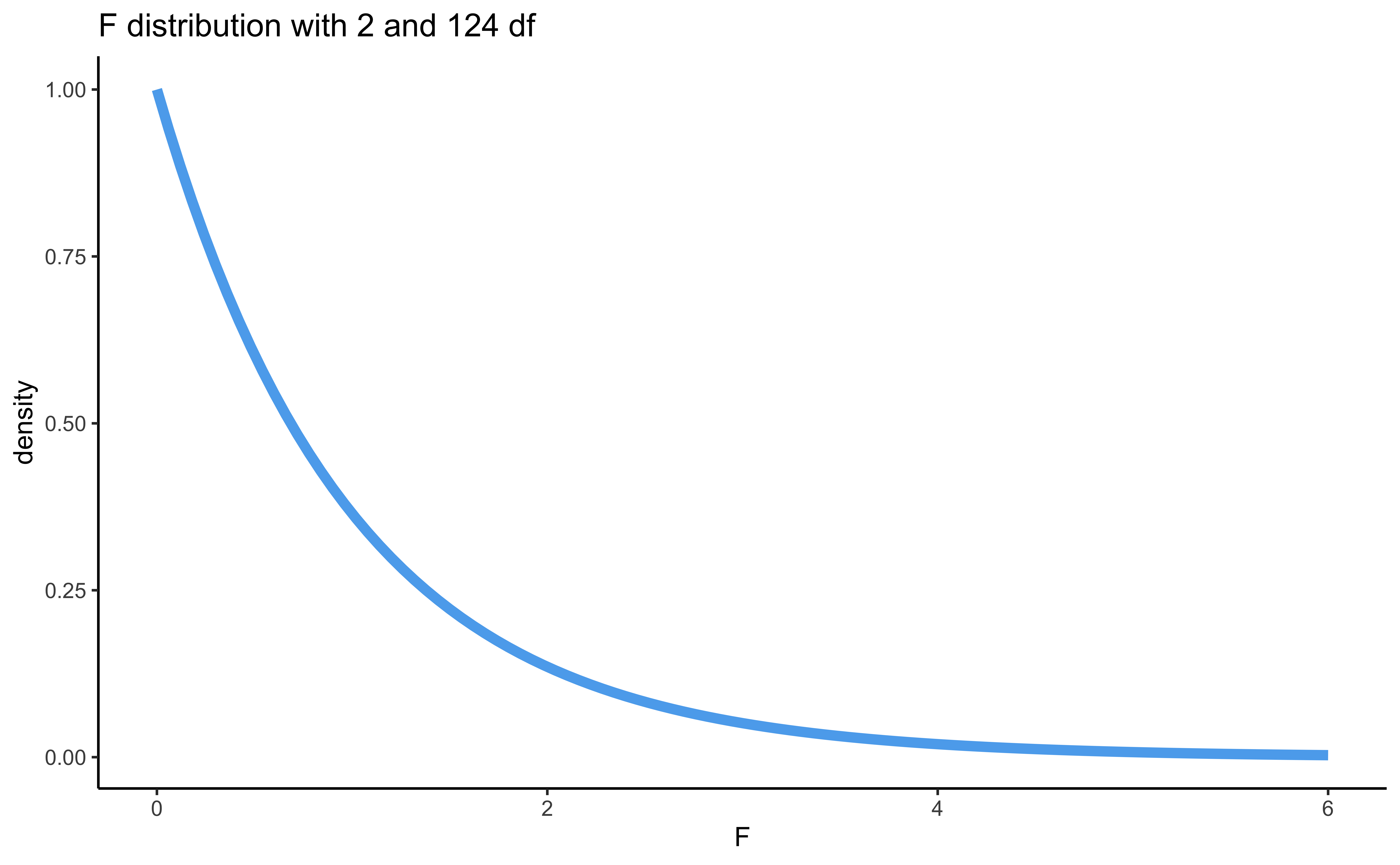
\[ \text{P-value} = \text{Pr}(F > \text{F Stat}) \]
Test for overall significance: Conclusion
\[ \begin{aligned} &H_0: \beta_1 = \beta_2 = 0\\ &H_a: \beta_j \neq 0 \text{ for at least one }j \end{aligned} \]
| Source | Df | Sum Sq | Mean Sq | F Stat | Pr(> F) |
|---|---|---|---|---|---|
| Model | 2 | 7138.591 | 3569.296 | 26.628 | 0 |
| Residuals | 124 | 16621.344 | 134.043 | ||
| Total | 126 | 23759.935 |
What is the conclusion from this hypothesis test?
Recap
Introduced statistical inference in the context of regression
Described the assumptions for regression
Connected the distribution of residuals and inferential procedures
Conducted inference on a single coefficient
Conducted inference on the overall regression model