Properties of estimators
Oct 01, 2024
Announcements
Project Proposal due Thursday, October 3 at 11:59pm
Lab 03 due Thursday, October 3 at 11:59pm
HW 02 due Thursday, October 3 at 11:59pm (released after class)
Exam 01: Tuesday, October 8 (in class + take-home)
Lecture recordings available until the start of the in-class exam (Link on side bar of webpage)
Exam review on Thursday
Monday’s lab: Exam office hours
No office hours while take-home exam is out
Topics
- Properties of the least squares estimator
Note
This is not a mathematical statistics class. There are semester-long courses that will go into these topics in much more detail; we will barely scratch the surface in this course.
Our goals are to understand
Estimators have properties
A few properties of the least squares estimator and why they are useful
Properties of \(\hat{\boldsymbol{\beta}}\)
Motivation
We have discussed how to use least squares to find an estimator of \(\hat{\boldsymbol{\beta}}\)
How do we know whether our least-squares estimator is a “good” estimator?
When we consider what makes an estimator “good”, we’ll look at three criteria:
- Bias
- Variance
- Mean squared error
We’ll take a look at these and motivate why we might prefer using least squares to compute \(\hat{\boldsymbol{\beta}}\) versus other methods
Bias and variance
Suppose you are throwing darts at a target
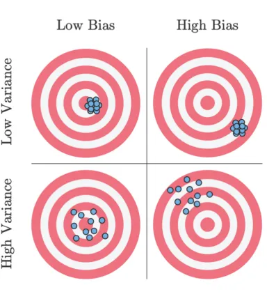
Ideal scenario: Darts are clustered around the target (unbiased and low variance)
Worst case scenario: Darts are widely spread out and systematically far from the target (high bias and high variance)
Acceptable scenario: There’s some trade-off between the bias and variance.
Properties of \(\hat{\boldsymbol{\beta}}\)
Finite sample ( \(n\) ) properties
Unbiased estimator
Best Linear Unbiased Estimator (BLUE)
Infinite sample ( \(n \rightarrow \infty\) ) properties
Consistent estimator
Efficient estimator
Finite sample properties
Unbiased estimator
The bias of an estimator is the difference between the estimator’s expected value and the true value of the parameter
Let \(\hat{\theta}\) be an estimator of the parameter \(\theta\). Then
\[ Bias(\hat{\theta}) = E(\hat{\theta}) - \theta \]
An estimator is unbiased if the bias is 0 and thus \(E(\hat{\theta}) = \theta\)
Unbiased estimator
\[ \begin{aligned} E(\hat{\boldsymbol{\beta}}) &= E[(\mathbf{X}^T\mathbf{X})^{-1}\mathbf{X}^T\mathbf{y}] \\[8pt] & = E[(\mathbf{X}^T\mathbf{X})^{-1}\mathbf{X}^T(\mathbf{X}\boldsymbol{\beta} + \mathbf{\epsilon})] \\[8pt] & = E[(\mathbf{X}^T\mathbf{X})^{-1}\mathbf{X}^T\mathbf{X}\boldsymbol{\beta}] + E[(\mathbf{X}^T\mathbf{X})^{-1}\mathbf{X}^T\boldsymbol{\epsilon}]\\[8pt] & = \boldsymbol{\beta} + (\mathbf{X}^T\mathbf{X})^{-1}\mathbf{X}^TE(\boldsymbol{\epsilon}) \\[8pt] & = \boldsymbol{\beta} \end{aligned} \]
The least-squares estimator \(\hat{\boldsymbol{\beta}}\) is an unbiased estimator of \(\boldsymbol{\beta}\)
Variance of \(\hat{\boldsymbol{\beta}}\)
\[ \begin{aligned} Var(\hat{\boldsymbol{\beta}}) &= Var((\mathbf{X}^T\mathbf{X})^{-1}\mathbf{X}^T\mathbf{y}) \\[8pt] & = [(\mathbf{X}^T\mathbf{X})^{-1}\mathbf{X}^T]Var(\mathbf{y})[(\mathbf{X}^T\mathbf{X})^{-1}\mathbf{X}^T]^T \\[8pt] & = [(\mathbf{X}^T\mathbf{X})^{-1}\mathbf{X}^T]\sigma^2_{\epsilon}\mathbf{I}[\mathbf{X}(\mathbf{X}^T\mathbf{X})^{-1}] \\[8pt] & = \sigma^2_{\epsilon}[(\mathbf{X}^T\mathbf{X})^{-1}\mathbf{X}^T\mathbf{X}(\mathbf{X}^T\mathbf{X})^{-1}] \\[8pt] & = \sigma^2_{\epsilon}(\mathbf{X}^T\mathbf{X})^{-1} \end{aligned} \]
“Linear” regression model
What does it mean for a model to be a “linear” regression model?
Linear regression models are linear in the parameters, i.e. given an observation \(y_i\)
\[ y_i = \beta_0 + \beta_1f_1(x_{i1}) + \dots + \beta_pf_p(x_{ip}) + \epsilon_i \]
The functions \(f_1, \ldots, f_p\) can be non-linear as long as \(\beta_0, \beta_1, \ldots, \beta_p\) are linear in \(Y\)
Gauss-Markov Theorem
The least-squares estimator of \(\boldsymbol{\beta}\) in the model \(\mathbf{y} = \mathbf{X}\boldsymbol{\beta} + \boldsymbol{\epsilon}\) is given by \(\hat{\boldsymbol{\beta}}\). Given the errors have mean \(\mathbf{0}\) and variance \(\sigma^2_{\epsilon}\mathbf{I}\) , then \(\hat{\boldsymbol{\beta}}\) is BLUE (best linear unbiased estimator).
“Best” means \(\hat{\boldsymbol{\beta}}\) has the smallest variance among all linear unbiased estimators for \(\boldsymbol{\beta}\) .
Gauss-Markov Theorem Proof
Suppose \(\tilde{\boldsymbol{\beta}}\) is another linear unbiased estimator of \(\boldsymbol{\beta}\) that can be expressed as \(\tilde{\boldsymbol{\beta}} = \mathbf{Cy}\) , such that \(\hat{\mathbf{y}} = \mathbf{X}\tilde{\boldsymbol{\beta}} = \mathbf{XCy}\)
Let \(\mathbf{C} = (\mathbf{X}^T\mathbf{X})^{-1}\mathbf{X}^T + \mathbf{B}\) for a non-zero matrix \(\mathbf{B}\).
What is the dimension of \(\mathbf{B}\)?
Gauss-Markov Theorem Proof
\[ \tilde{\boldsymbol{\beta}} = \mathbf{Cy} = ((\mathbf{X}^T\mathbf{X})^{-1}\mathbf{X}^T + \mathbf{B})\mathbf{y} \]
We need to show
\(\tilde{\boldsymbol{\beta}}\) is unbiased
\(Var(\tilde{\boldsymbol{\beta}}) > Var(\hat{\boldsymbol{\beta}})\)
Gauss-Markov Theorem Proof
\[ \begin{aligned} E(\tilde{\boldsymbol{\beta}}) & = E[((\mathbf{X}^T\mathbf{X})^{-1}\mathbf{X}^T + \mathbf{B})\mathbf{y}] \\ & = E[((\mathbf{X}^T\mathbf{X})^{-1}\mathbf{X}^T + \mathbf{B})(\mathbf{X}\boldsymbol{\beta} + \boldsymbol{\epsilon})] \\ & = E[((\mathbf{X}^T\mathbf{X})^{-1}\mathbf{X}^T + \mathbf{B})(\mathbf{X}\boldsymbol{\beta})] \\ & = ((\mathbf{X}^T\mathbf{X})^{-1}\mathbf{X}^T + \mathbf{B})(\mathbf{X}\boldsymbol{\beta}) \\ & = (\mathbf{I} + \mathbf{BX})\boldsymbol{\beta} \end{aligned} \]
What assumption(s) of the Gauss-Markov Theorem did we use?
What must be true for \(\tilde{\boldsymbol{\beta}}\) to be unbiased?
Gauss-Markov Theorem Proof
\(\mathbf{BX}\) must be the \(\mathbf{0}\) matrix (dimension = \((p+1) \times (p+1)\)) in order for \(\tilde{\boldsymbol{\beta}}\) to be unbiased
Now we need to find \(Var(\tilde{\boldsymbol{\beta}})\) and see how it compares to \(Var(\hat{\boldsymbol{\beta}})\)
Gauss-Markov Theorem Proof
\[ \begin{aligned} Var(\tilde{\boldsymbol{\beta}}) &= Var[((\mathbf{X}^T\mathbf{X})^{-1}\mathbf{X}^T + \mathbf{B})\mathbf{y}] \\[8pt] & = ((\mathbf{X}^T\mathbf{X})^{-1}\mathbf{X}^T + \mathbf{B})Var(\mathbf{y})((\mathbf{X}^T\mathbf{X})^{-1}\mathbf{X}^T + \mathbf{B})^T \\[8pt] & = \small{\sigma^2_{\epsilon}[(\mathbf{X}^T\mathbf{X})^{-1}\mathbf{X}^T\mathbf{X}(\mathbf{X}^T\mathbf{X})^{-1} + (\mathbf{X}^T\mathbf{X})^{-1}\mathbf{X}^T \mathbf{B}^T + \mathbf{BX}(\mathbf{X}^T\mathbf{X})^{-1} + \mathbf{BB}^T]}\\[8pt] & = \sigma^2_\epsilon(\mathbf{X}^T\mathbf{X})^{-1} + \sigma^2_{\epsilon}\mathbf{BB}^T\end{aligned} \]
What assumption(s) of the Gauss-Markov Theorem did we use?
Gauss-Markov Theorem Proof
We have
\[ Var(\tilde{\boldsymbol{\beta}}) = \sigma^2_{\epsilon}(\mathbf{X}^T\mathbf{X})^{-1} + \sigma^2_\epsilon \mathbf{BB}^T \]
We know that \(\sigma^2_{\epsilon}\mathbf{BB}^T \geq \mathbf{0}\).
When is \(\sigma^2_{\epsilon}\mathbf{BB}^T = \mathbf{0}\)?
Therefore, we have shown that \(Var(\tilde{\boldsymbol{\beta}}) > Var(\hat{\boldsymbol{\beta}})\) and have completed the proof.
Gauss-Markov Theorem
The least-squares estimator of \(\boldsymbol{\beta}\) in the model \(\mathbf{y} = \mathbf{X}\boldsymbol{\beta} + \boldsymbol{\epsilon}\) is given by \(\hat{\boldsymbol{\beta}}\). Given the errors have mean \(\mathbf{0}\) and variance \(\sigma^2_{\epsilon}\mathbf{I}\) , then \(\hat{\boldsymbol{\beta}}\) is BLUE (best linear unbiased estimator).
“Best” means \(\hat{\boldsymbol{\beta}}\) has the smallest variance among all linear unbiased estimators for \(\boldsymbol{\beta}\) .
Properties of \(\hat{\boldsymbol{\beta}}\)
Finite sample ( \(n\) ) properties
Unbiased estimator ✅
Best Linear Unbiased Estimator (BLUE) ✅
Infinite sample ( \(n \rightarrow \infty\) ) properties
Consistent estimator
Efficient estimator
Infinite sample properties
Mean squared error
The mean squared error (MSE) is the squared difference between the estimator and parameter.
Let \(\hat{\theta}\) be an estimator of the parameter \(\theta\). Then
\[ \begin{aligned} MSE(\hat{\theta}) &= E[(\hat{\theta} - \theta)^2] \\ & = E(\hat{\theta}^2 - 2\hat{\theta}\theta + \theta^2) \\ & = E(\hat{\theta}^2) - 2\theta E(\hat{\theta}) + \theta^2 \\ & = \underbrace{E(\hat{\theta}^2) - E(\hat{\theta})^2}_{Var(\hat{\theta})} + \underbrace{E(\hat{\theta})^2 - 2\theta E(\hat{\theta}) + \theta^2}_{Bias(\theta)^2} \end{aligned} \]
Mean squared error
\[ MSE(\hat{\theta}) = Var(\hat{\theta}) + Bias(\hat{\theta})^2 \]
The least-squares estimator \(\hat{\boldsymbol{\beta}}\) is unbiased, so \[MSE(\hat{\boldsymbol{\beta}}) = Var(\hat{\boldsymbol{\beta}})\]
Consistency
An estimator \(\hat{\theta}\) is a consistent estimator of a parameter \(\theta\) if it converges in probability to \(\theta\). Given a sequence of estimators \(\hat{\theta}_1, \hat{\theta}_2, . . .\), then for every \(\epsilon > 0\),
\[ \displaystyle \lim_{n\to\infty} P(|\hat{\theta}_n - \theta| \geq \epsilon) = 0 \]
This means that as the sample size goes to \(\infty\) (and thus the sample information gets better and better), the estimator will be arbitrarily close to the parameter with high probability.
Why is this a useful property of an estimator?
Consistency
Important
Theorem
An estimator \(\hat{\theta}\) is a consistent estimator of the parameter \(\theta\) if the sequence of estimators \(\hat{\theta}_1, \hat{\theta}_2, \ldots\) satisfies
\(\lim_{n \to \infty} Var(\hat{\theta}) = 0\)
\(\lim_{n \to \infty} Bias(\hat{\theta}) = 0\)
Consistency of \(\hat{\boldsymbol{\beta}}\)
\(Bias(\hat{\boldsymbol{\beta}}) = \mathbf{0}\), so \(\lim_{n \to \infty} Bias(\hat{\boldsymbol{\beta}}) = \mathbf{0}\)
Now we need to show that \(\lim_{n \to \infty} Var(\hat{\boldsymbol{\beta}}) = \mathbf{0}\)
What is \(Var(\hat{\boldsymbol{\beta}})\)?
Does \(Var(\hat{\boldsymbol{\beta}}) \to \mathbf{0}\) as \(n \to \infty\)?
Efficiency
The efficiency of an estimator is concerned with the asymptotic variance of an estimator.
The estimator with the smallest variance is considered the most efficient.
By the Gauss-Markov Theorem, we have shown that the least-squares estimator is the most efficient among linear unbiased estimators.
Recap
Finite sample ( \(n\) ) properties
Unbiased estimator ✅
Best Linear Unbiased Estimator (BLUE) ✅
Infinite sample ( \(n \rightarrow \infty\) ) properties
Consistent estimator ✅
Efficient estimator ✅