Variable transformations
Oct 24, 2024
Announcements
Exam corrections (optional) due TODAY at 11:59pm on Canvas
Lab 04 due TODAY at 11:59pm
Team Feedback (from TEAMMATES) due TODAY at 11:59pm
Mid semester survey (strongly encouraged!) by TODAY at 11:59pm
HW 03 due Thursday October 31 at 11:59pm (released after class)
Looking ahead
Project: Exploratory data analysis due October 31
Statistics experience due Tuesday, November 26
Exam weighting
No curves on individual exam grades
Exams will be weighted to reflect significant progress throughout semester. There are 2 scenarios:
If Exam 02 score is at least 5 (out of 50) points greater than the Exam 01 score (before corrections), Exam 01 is 13% and Exam 02 is 27% of the final course grade
Otherwise, the exams are 20% each as stated in the syllabus.
Computing set up
Topics
- Variable transformations
Variable transformations
Data: Respiratory Rate vs. Age
A high respiratory rate can potentially indicate a respiratory infection in children. In order to determine what indicates a “high” rate, we first want to understand the relationship between a child’s age and their respiratory rate.
The data contain the respiratory rate for 618 children ages 15 days to 3 years. It was obtained from the Sleuth3 R package and is originally form a 1994 publication “Reference Values for Respiratory Rate in the First 3 Years of Life”.
Variables:
Age: age in monthsRate: respiratory rate (breaths per minute)
Rate vs. Age
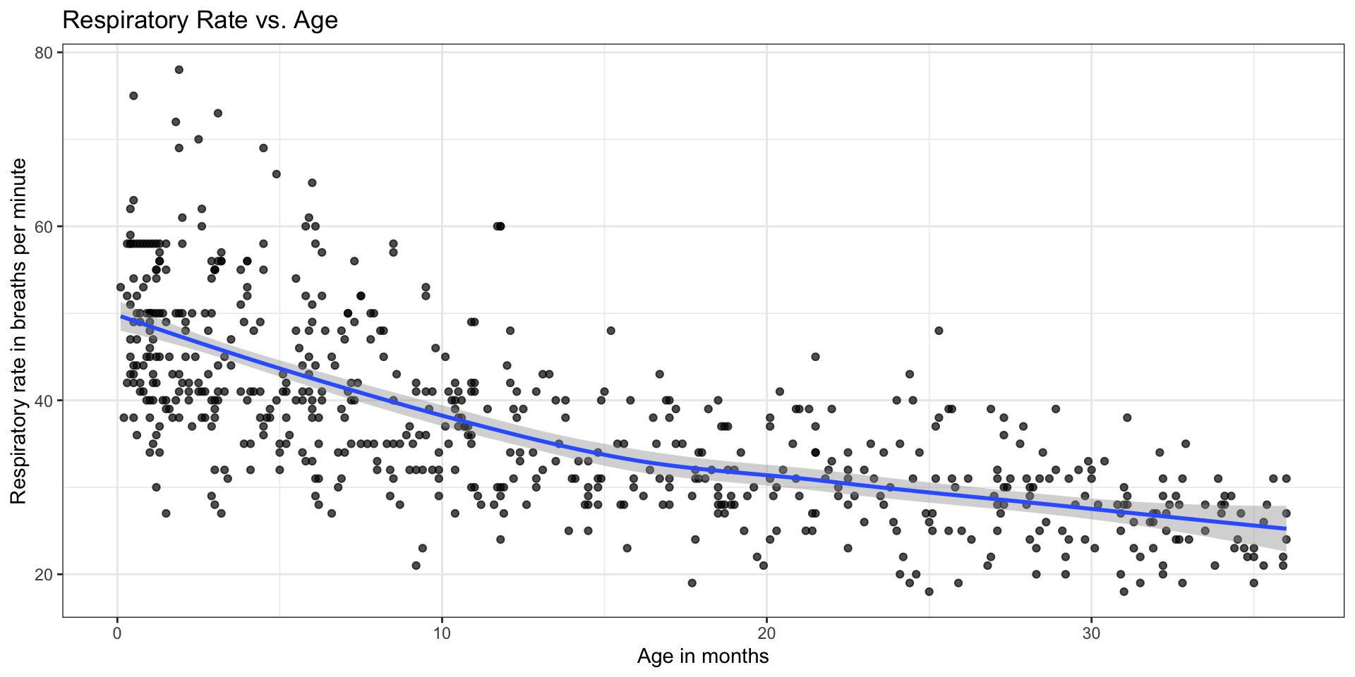
Model 1: Rate vs. Age
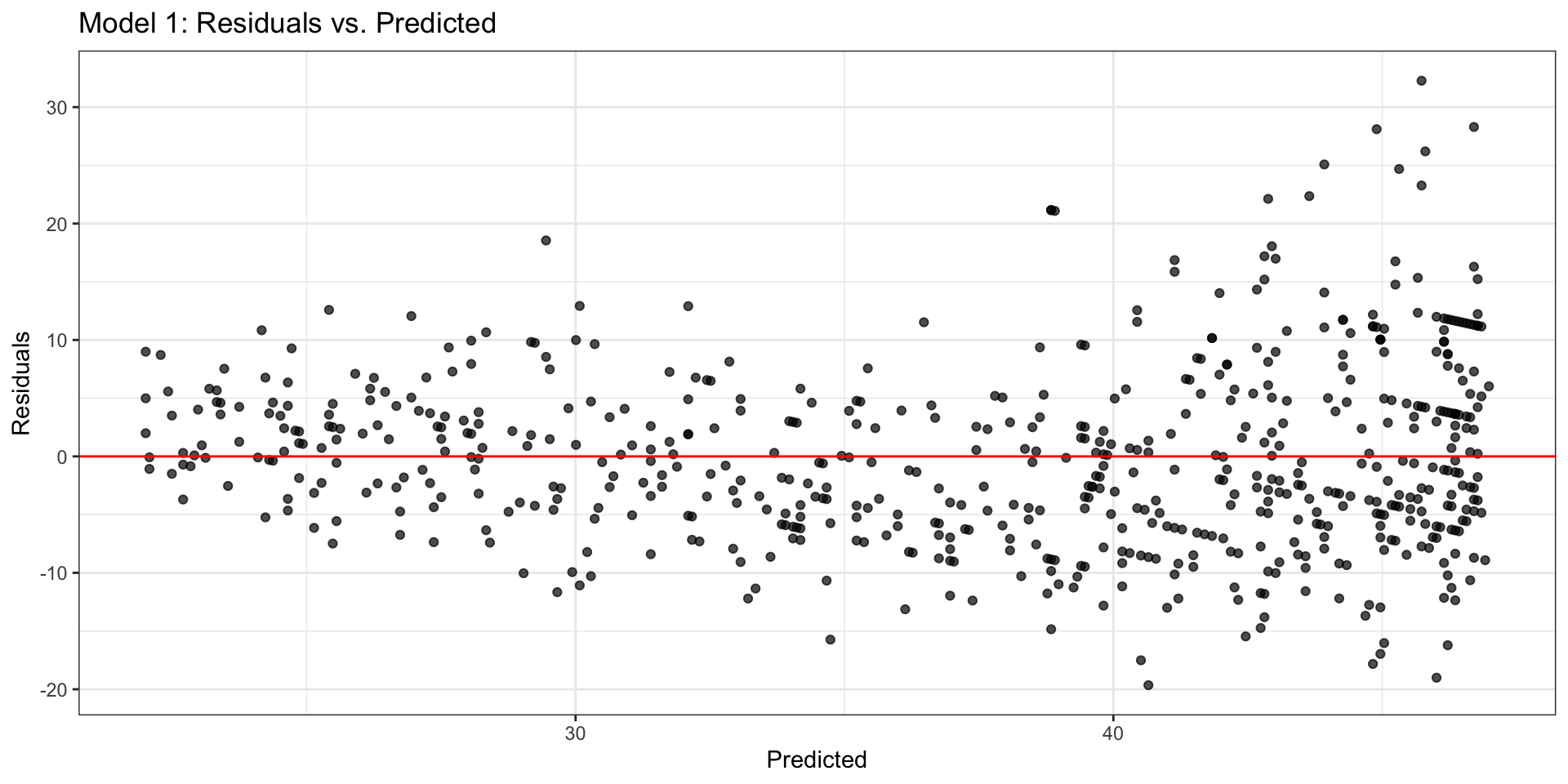
Model 1: Residuals
Consider different transformations…
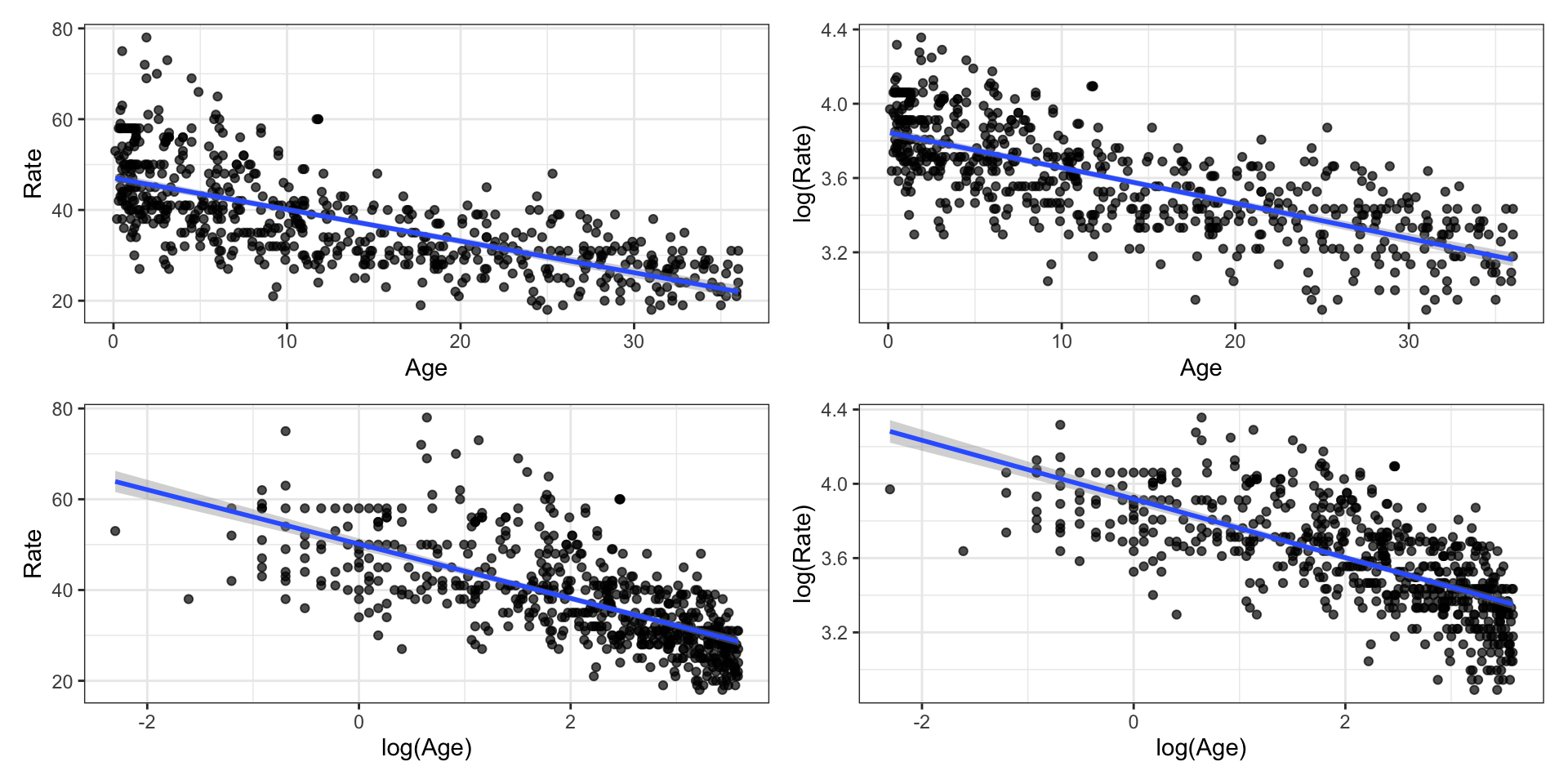
Transformation on \(Y\)
Identifying a need to transform Y
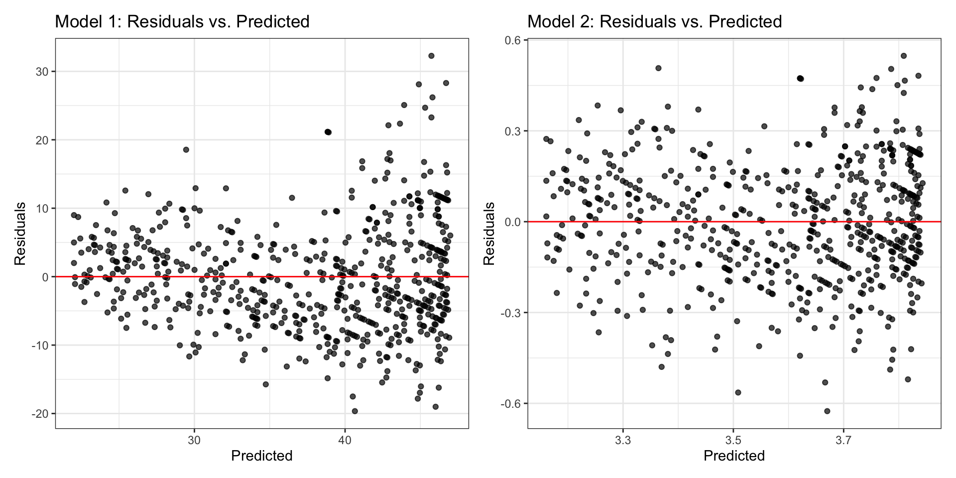
Typically, a “fan-shaped” residual plot indicates the need for a transformation of the response variable Y
There are multiple ways to transform a variable, e.g., Y, 1/Y, log(Y)
log(Y) the most straightforward to interpret, so we use that transformation when possible
When building a model:
Choose a transformation and build the model on the transformed data
Reassess the residual plots
If the residuals plots did not sufficiently improve, try a new transformation!
Log transformation on \(Y\)
- If we apply a log transformation to the response variable, we want to estimate the parameters for the statistical model
\[ \log(y_i) = \beta_0+ \beta_1 x_{i1} + \dots +\beta_px_{ip} + \epsilon_i, \hspace{10mm} \epsilon \sim N(0,\sigma^2_\epsilon) \]
- The regression equation is
\[\widehat{\log(y_i)} = \hat{\beta}_0+ \hat{\beta}_1 x_{i1} + \dots + \hat{\beta}_px_{ip}\]
Log transformation on \(Y\)
We want to interpret the model in terms of the original variable \(Y\), not \(\log(Y)\), so we need to write the regression equation in terms of \(Y\)
\[\begin{align}\hat{y_i} &= \exp\{\hat{\beta}_0 + \hat{\beta}_1 x_{i1} + \dots + \hat{\beta}_Px_{ip}\}\\ &= \exp\{\hat{\beta}_0\}\exp\{\hat{\beta}_1x_{i1}\}\dots\exp\{\hat{\beta}_px_{ip}\}\end{align}\]
Note
The predicted value \(\hat{y_i}\) is the predicted median of \(Y\). Note, when the distribution of \(y_i|x_1, \ldots, x_p\) is symmetric, then the median equals the mean. (See notes at the end for more details)
Model interpretation
\[\begin{align}\hat{y_i} &= \exp\{\hat{\beta}_0 + \hat{\beta}_1 x_{1p} + \dots + \hat{\beta}_Px_{ip}\}\\ &= \exp\{\hat{\beta}_0\}\exp\{\hat{\beta}_1x_{i1}\}\dots\exp\{\hat{\beta}_px_{ip}\}\end{align}\]
Intercept: When \(x_{i1} = \dots = x_{ip} =0\), \(y_i\) is expected to be \(\exp\{\hat{\beta}_0\}\)
Slope: For every one unit increase in \(x_{ij}\), \(y_{i}\) is expected to multiply by a factor of \(\exp\{\hat{\beta}_j\}\), holding all else constant
Why is the interpretation in terms of a multiplicative change?
Model 2: log(Rate) vs. Age
| term | estimate | std.error | statistic | p.value |
|---|---|---|---|---|
| (Intercept) | 3.845 | 0.013 | 304.500 | 0 |
| Age | -0.019 | 0.001 | -25.839 | 0 |
Interpret the intercept in terms of (1)
log(Rate)and (2)Rate.Interpret the effect of
Agein terms of (1)log(Rate)and (2)Rate.
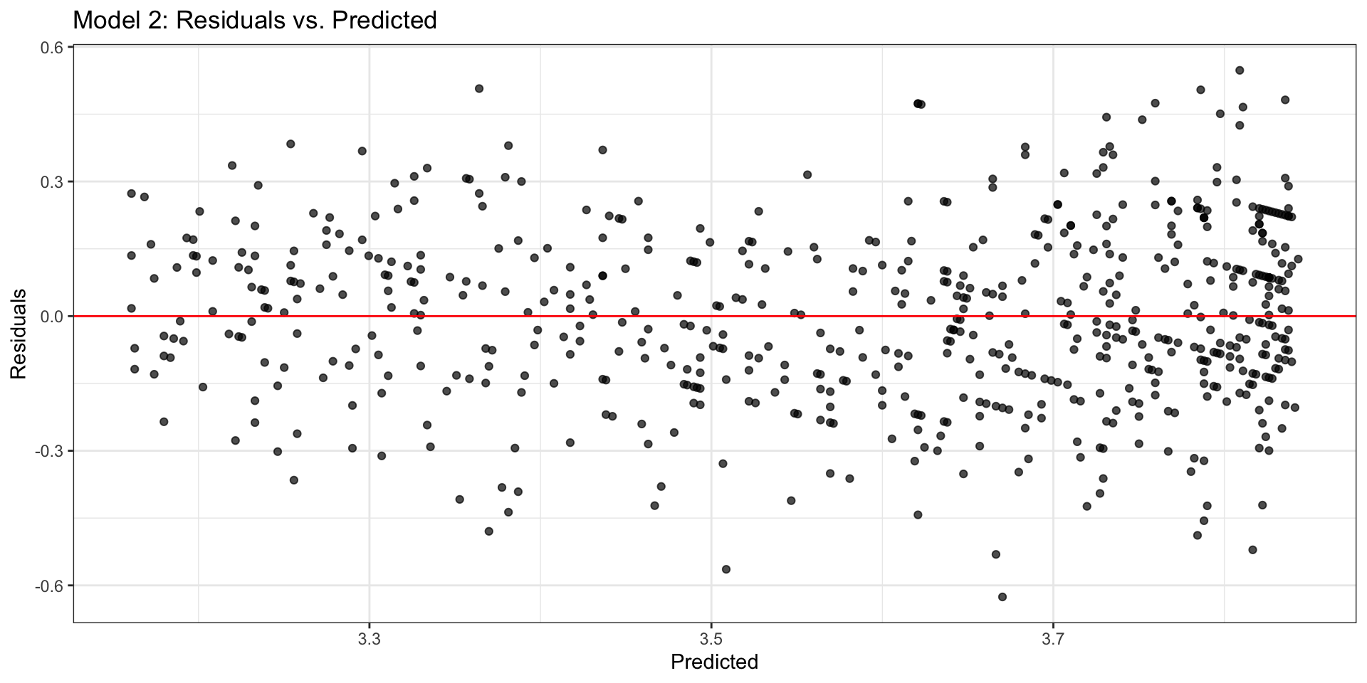
Model 2: Residuals
Compare residual plots
Log transformation on a predictor variable
Log Transformation on \(X\)
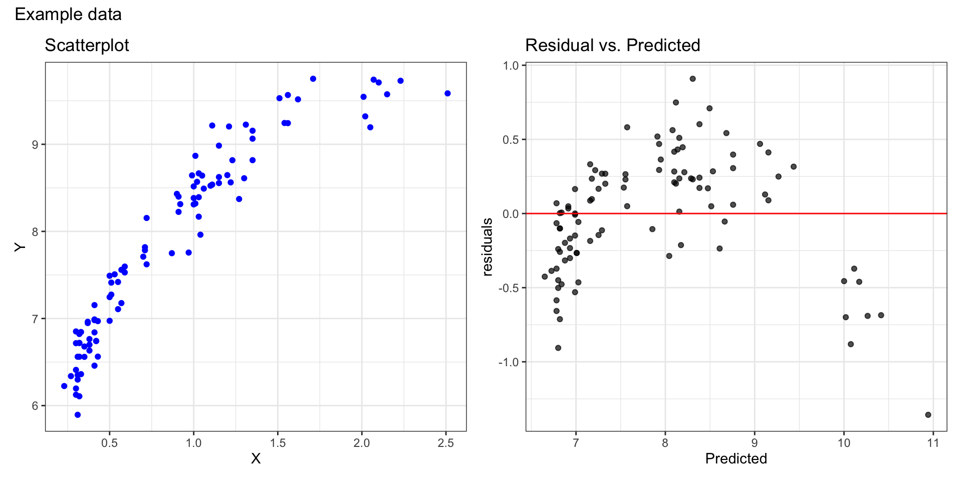
Try a transformation on \(X\) if the scatterplot shows some curvature but the variance is constant for all values of \(X\)
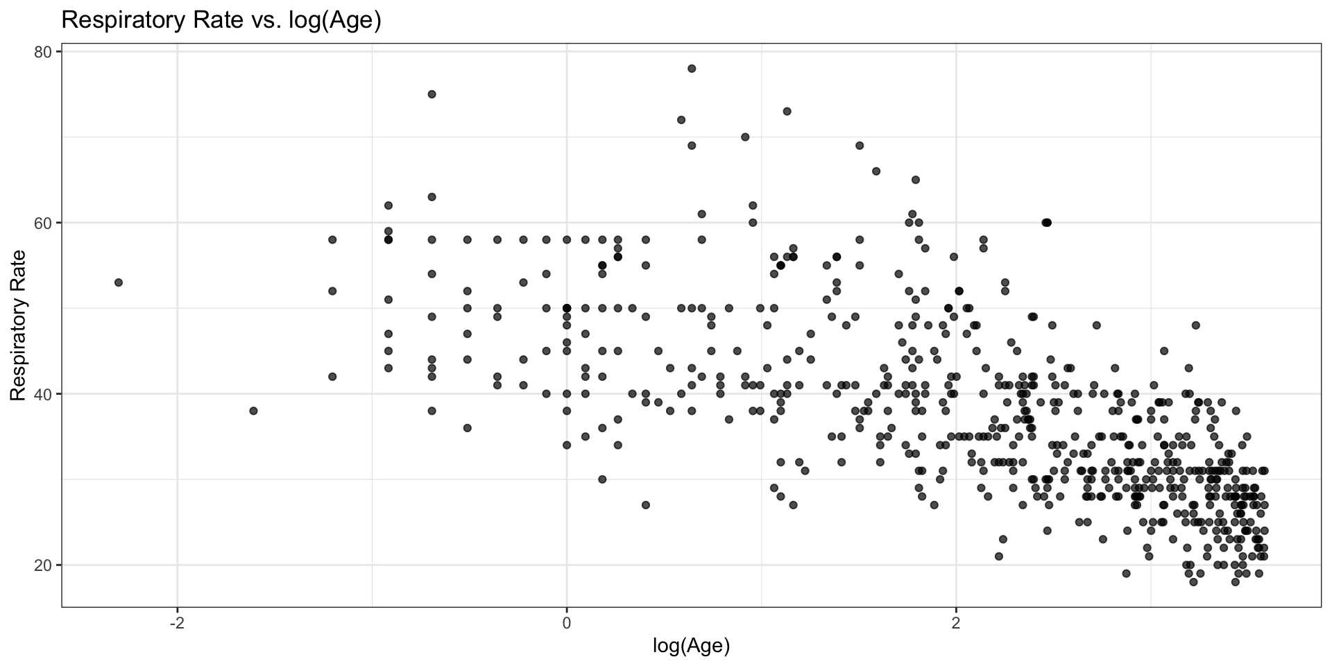
Rate vs. log(Age)
Model with Transformation on \(X\)
Suppose we have the following regression equation:
\[\hat{y}_i = \hat{\beta}_0 + \hat{\beta}_1 \log(x_i)\]
Intercept: When \(x_i = 1\) \((\log(x_i) = 0)\), \(y_i\) is expected to be \(\hat{\beta}_0\) (i.e. the mean of \(y_i\) is \(\hat{\beta}_0\))
Slope: When \(x_i\) is multiplied by a factor of \(\mathbf{C}\), the mean of \(y_i\) is expected to change by \(\hat{\beta}_1\log(C)\) units
- Example: when \(x_i\) is multiplied by a factor of 2, \(y_i\) is expected to increase by \(\hat{\beta}_1\log(2)\) units
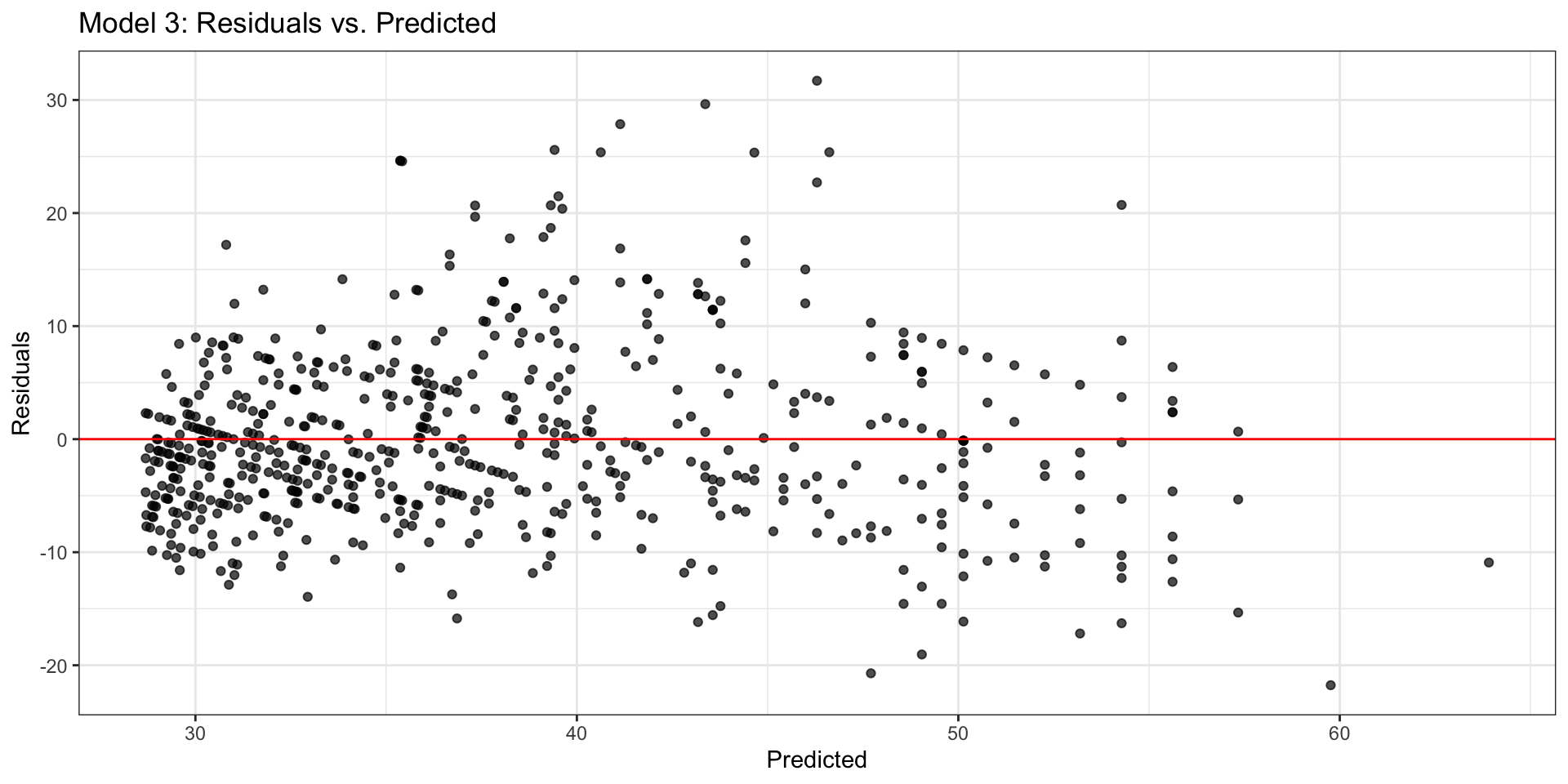
Model 3: Rate vs. log(Age)
| term | estimate | std.error | statistic | p.value |
|---|---|---|---|---|
| (Intercept) | 50.135 | 0.632 | 79.330 | 0 |
| log_age | -5.982 | 0.263 | -22.781 | 0 |
Interpret the slope and intercept in the context of the data.
Model 3: Residuals
Choose a model
Recall the goal of the analysis:
In order to determine what indicates a “high” rate, we first want to understand the relationship between a child’s age and their respiratory rate.
Which is the preferred metric to compare the models - \(R^2\) or RMSE?
Compare models
| Rate vs. Age | log(Rate) vs. Age | Rate vs. log(Age) |
|---|---|---|
| 0.477 | 0.52 | 0.457 |
Which model would you choose?
Learn more
See Log Transformations in Linear Regression for more details about interpreting regression models with log-transformed variables.
Recap
- Introduced variable transformations
