Model comparison

Prof. Maria Tackett

Oct 29, 2024

Announcements

HW 03 due Thursday at 11:59pm
Project: Exploratory data analysis due Thursday at 11:59pm
Looking ahead
- Project presentations November 11
- Statistics experience due Tuesday, November 26

Computing set up

# load packages
library(tidyverse)  
library(tidymodels)  
library(knitr)       
library(patchwork)
library(kableExtra) # for formatting tables

# set default theme in ggplot2
ggplot2::theme_set(ggplot2::theme_bw())

Topics

ANOVA for Multiple Linear Regression
Nested (Partial) F Test
AIC & BIC

Restaurant tips

What affects the amount customers tip at a restaurant?

Response:
- Tip: amount of the tip
Predictors:
- Party: number of people in the party
- Meal: time of day (Lunch, Dinner, Late Night)
- Age: age category of person paying the bill (Yadult, Middle, SenCit)

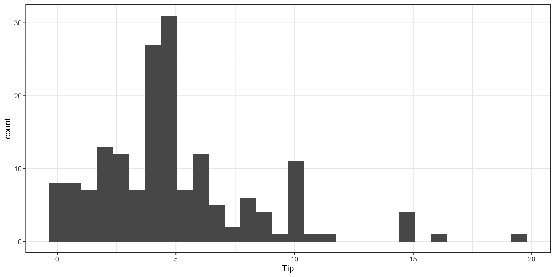
Response Variable

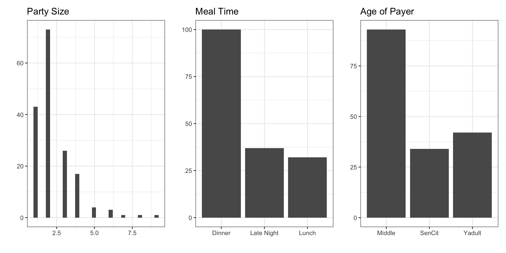
Predictor Variables

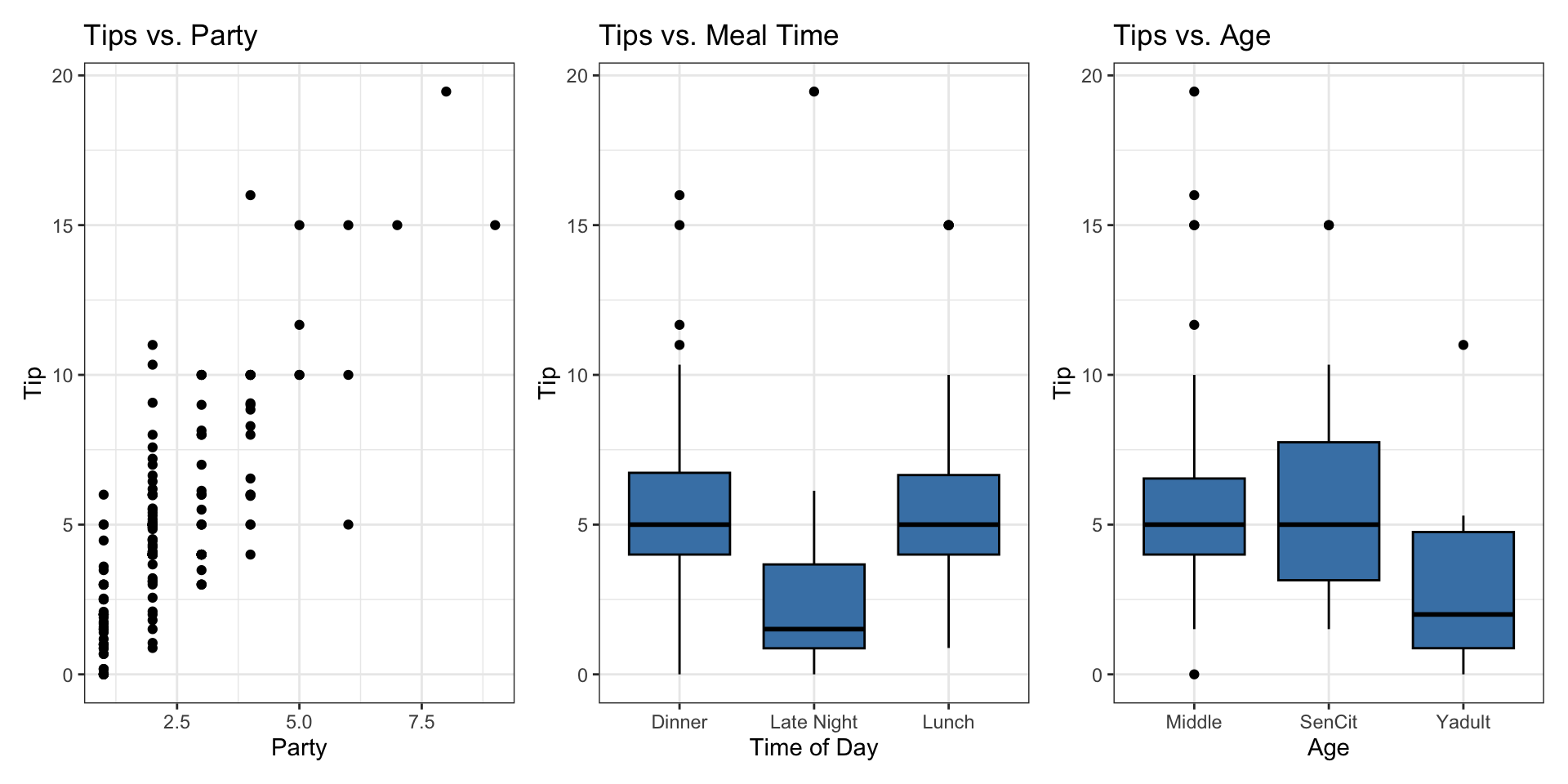
Response vs. Predictors

Restaurant tips: model

model1 <- lm(Tip ~ Party +  Age , data = tips)
tidy(model1, conf.int = TRUE) |>
  kable(format = "markdown", digits=3)

term	estimate	std.error	statistic	p.value	conf.low	conf.high
(Intercept)	0.838	0.397	2.112	0.036	0.055	1.622
Party	1.837	0.124	14.758	0.000	1.591	2.083
AgeSenCit	0.379	0.410	0.925	0.356	-0.430	1.189
AgeYadult	-1.009	0.408	-2.475	0.014	-1.813	-0.204

Is this the best model to explain variation in Tips?

Test for overall significance

Test for overall significance: Hypotheses

We can conduct a hypothesis test using the ANOVA table to determine if there is at least one non-zero coefficient in the model

\[ \begin{aligned} &H_0: \beta_1 = \dots = \beta_p = 0\\ &H_a: \beta_j \neq 0 \text{ for at least one }j \end{aligned} \]

For the tips data:\[ \begin{aligned} &H_0: \beta_1 = \beta_2 = \beta_3 = 0\\ &H_a: \beta_j \neq 0 \text{ for at least one }j \end{aligned} \]

Test for overall significance: Test statistic

Source	Df	Sum Sq	Mean Sq	F Stat	Pr(> F)
Model	3	1226.664	408.888	98.284	0
Residuals	165	686.444	4.16
Total	168	1913.108

Test statistic: Ratio of explained to unexplained variability

\[ F = \frac{\text{Mean Square Model}}{\text{Mean Square Residuals}} \]

The test statistic follows an \(F\) distribution with \(p\) and \(n - p - 1\) degrees of freedom

Test for overall significance: P-value

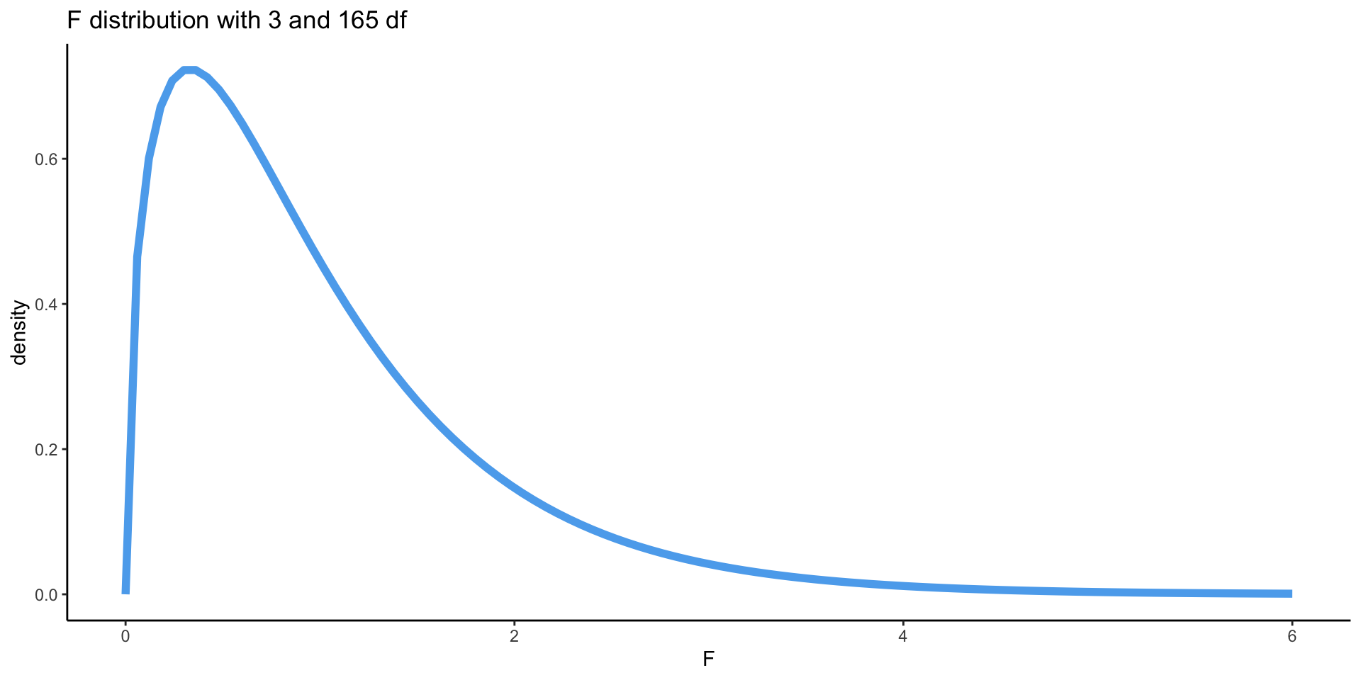
\[ \text{P-value} = \text{Pr}(F > \text{F Stat}) \]

Test for overall significance: Conclusion

\[ \begin{aligned} &H_0: \beta_1 = \beta_2 = \beta_3 = 0\\ &H_a: \beta_j \neq 0 \text{ for at least one }j \end{aligned} \]

Source	Df	Sum Sq	Mean Sq	F Stat	Pr(> F)
Model	3	1226.664	408.888	98.284	0
Residuals	165	686.444	4.16
Total	168	1913.108

What is the conclusion from this hypothesis test?

Why use overall F test?

Why do we use overall F test instead of just looking at the test for individual coefficients?¹

Suppose we have a model such that \(p = 100\) and \(H_0: \beta_1 = \dots = \beta_{100} = 0\) is true

About 5% of the p-values for individual coefficients will be below 0.05 by chance.
So we expect to see 5 small p-values if even no linear association actually exists.
Therefore, it is very likely we will see at least one small p-value by chance.
The F-test does not have this problem, because it accounts for the number of predictors. There is only a 5% chance we will get a p-value below 0.05, if a linear relationship truly does not exist.

Testing subset of coefficients

Sometimes we want to test whether a subset of coefficients are all equal to 0
This is often the case when we want test
- whether a categorical variable with \(k\) levels is a significant predictor of the response
- whether the interaction between a categorical and quantitative variable is significant
To do so, we will use the Nested (Partial) F-test

Nested (Partial) F Test

Suppose we have a full and reduced model:

\[\begin{aligned}&\text{Full}: y = \beta_0 + \beta_1 x_1 + \dots + \beta_q x_q + \beta_{q+1} x_{q+1} + \dots \beta_p x_p \\ &\text{Reduced}: y = \beta_0 + \beta_1 x_1 + \dots + \beta_q x_q\end{aligned}\]

We want to test whether any of the variables \(x_{q+1}, x_{q+2}, \ldots, x_p\) are significant predictors. To do so, we will test the hypothesis:

\[\begin{aligned}&H_0: \beta_{q+1} = \beta_{q+2} = \dots = \beta_p = 0 \\ &H_a: \text{at least one }\beta_j \text{ is not equal to 0}\end{aligned}\]

Nested F Test

The test statistic for this test is

\[F = \frac{(SSR_{reduced} - SSR_{full})\big/\text{# predictors tested}}{SSR_{full}\big/(n-p_{full}-1)}\]

Calculate the p-value using the F distribution with df1 = # predictors tested and df2 = \((n-p_{full}-1)\)

Is `Meal` a significant predictor of tips?

term	estimate
(Intercept)	1.254
Party	1.808
AgeSenCit	0.390
AgeYadult	-0.505
MealLate Night	-1.632
MealLunch	-0.612

Tips: Nested F test

\[\begin{aligned}&H_0: \beta_{late night} = \beta_{lunch} = 0\\ &H_a: \text{ at least one }\beta_j \text{ is not equal to 0}\end{aligned}\]

reduced <- lm(Tip ~ Party + Age, data = tips)

full <- lm(Tip ~ Party + Age + Meal, data = tips)

#Nested F test in R
anova(reduced, full)

Tips: Nested F test

Res.Df	RSS	Df	Sum of Sq	F	Pr(>F)
165	686.444	NA	NA	NA	NA
163	622.979	2	63.465	8.303	0

F Stat: \(\frac{(686.444 - 622.979)/2}{622.979/(169 - 5 - 1)} = 8.303\)

P-value: P(F > 8.303) = 0.0003 - calculated using an F distribution with 2 and 163 degrees of freedom

The data provide sufficient evidence to conclude that at least one coefficient associated with Meal is not zero. Therefore, Meal is a significant predictor of Tips.

Model with `Meal`

term	estimate	std.error	statistic	p.value	conf.low	conf.high
(Intercept)	1.254	0.394	3.182	0.002	0.476	2.032
Party	1.808	0.121	14.909	0.000	1.568	2.047
AgeSenCit	0.390	0.394	0.990	0.324	-0.388	1.168
AgeYadult	-0.505	0.412	-1.227	0.222	-1.319	0.308
MealLate Night	-1.632	0.407	-4.013	0.000	-2.435	-0.829
MealLunch	-0.612	0.402	-1.523	0.130	-1.405	0.181

Including interactions

Does the effect of Party differ based on the Meal time?

term	estimate
(Intercept)	1.276
Party	1.795
AgeSenCit	0.401
AgeYadult	-0.470
MealLate Night	-1.845
MealLunch	-0.461
Party:MealLate Night	0.111
Party:MealLunch	-0.050

Nested F test for interactions

Let’s use a Nested F test to determine if Party*Meal is statistically significant.

reduced <- lm(Tip ~ Party + Age + Meal, data = tips)

full <- lm(Tip ~ Party + Age + Meal + Meal * Party, 
           data = tips)

kable(anova(reduced, full), format = "markdown", digits = 3) |>
  row_spec(2, background = "#dce5b2")

Res.Df	RSS	Df	Sum of Sq	F	Pr(>F)
163	622.979	NA	NA	NA	NA
161	621.965	2	1.014	0.131	0.877

Final model for now

We conclude that the effect of Party does not differ based Meal. Therefore, we will use the original model that only included main effects.

term	estimate	std.error	statistic	p.value
(Intercept)	1.254	0.394	3.182	0.002
Party	1.808	0.121	14.909	0.000
AgeSenCit	0.390	0.394	0.990	0.324
AgeYadult	-0.505	0.412	-1.227	0.222
MealLate Night	-1.632	0.407	-4.013	0.000
MealLunch	-0.612	0.402	-1.523	0.130

Model comparison using AIC and BIC

Tips: Comparing models

Let’s compare two models:

model1 <- lm(Tip ~ Party + Age + Meal, data = tips)
glance(model1) |> select(r.squared, adj.r.squared)

# A tibble: 1 × 2
  r.squared adj.r.squared
      <dbl>         <dbl>
1     0.674         0.664

model2 <- lm(Tip ~ Party + Age + Meal + Day, data = tips)
glance(model2) |> select(r.squared, adj.r.squared)

# A tibble: 1 × 2
  r.squared adj.r.squared
      <dbl>         <dbl>
1     0.683         0.662

AIC & BIC

Akaike’s Information Criterion (AIC): \[AIC = n\log(SSR) + 2(p+1)\]

Schwarz’s Bayesian Information Criterion (BIC) \[BIC = n\log(SSR) + log(n)\times(p+1)\]

AIC & BIC

\[\begin{aligned} & AIC = \color{blue}{n\log(SSR)} \color{black}{ + 2(p+1)} \\ & BIC = \color{blue}{n\log(SSR)} \color{black}{+ \log(n)\times(p+1) }\end{aligned}\]

First Term: Generally decreases as p increases

AIC & BIC

\[\begin{aligned} & AIC = n\log(SSR) + \color{blue}{2(p+1)} \\ & BIC = n\log(SSR) + \color{blue}{\log(n)\times(p+1)} \end{aligned}\]

Second Term: Increases as p increases

Using AIC & BIC

\[\begin{aligned} & AIC = n\log(SSR) + \color{red}{2(p+1)} \\ & BIC = n\log(SSR) + \color{red}{\log(n)\times(p+1)} \end{aligned}\]

Choose model with the smaller value of AIC or BIC
If \(n \geq 8\), the penalty for BIC is larger than that of AIC, so BIC tends to favor more parsimonious models (i.e. models with fewer terms)

Tips: AIC & BIC

model1 <- lm(Tip ~ Party + Age + Meal, data = tips)
glance(model1) |> select(AIC, BIC)

# A tibble: 1 × 2
    AIC   BIC
  <dbl> <dbl>
1  714.  736.

model2 <- lm(Tip ~ Party + Age + Meal + Day, data = tips)
glance(model2) |> select(AIC, BIC)

# A tibble: 1 × 2
    AIC   BIC
  <dbl> <dbl>
1  720.  757.

Which model do you choose?

Parsimony and Occam’s razor

The principle of parsimony is attributed to William of Occam (early 14th-century English nominalist philosopher), who insisted that, given a set of equally good explanations for a given phenomenon, the correct explanation is the simplest explanation¹
Called Occam’s razor because he “shaved” his explanations down to the bare minimum
Parsimony in modeling:
- models should have as few parameters as possible
- linear models should be preferred to non-linear models
- experiments relying on few assumptions should be preferred to those relying on many
- models should be pared down until they are minimal adequate
- simple explanations should be preferred to complex explanations

In pursuit of Occam’s razor

Occam’s razor states that among competing hypotheses that predict equally well, the one with the fewest assumptions should be selected
Model selection follows this principle
We only want to add another variable to the model if the addition of that variable brings something valuable in terms of predictive power to the model
In other words, we prefer the simplest best model, i.e. parsimonious model

In pursuit of Occam’s razor

Occam’s razor states that among competing hypotheses that predict equally well, the one with the fewest assumptions should be selected
Model selection follows this principle
We only want to add another variable to the model if the addition of that variable brings something valuable in terms of predictive power to the model
In other words, we prefer the simplest best model, i.e. parsimonious model

Alternate views

Sometimes a simple model will outperform a more complex model . . . Nevertheless, I believe that deliberately limiting the complexity of the model is not fruitful when the problem is evidently complex. Instead, if a simple model is found that outperforms some particular complex model, the appropriate response is to define a different complex model that captures whatever aspect of the problem led to the simple model performing well.

Radford Neal - Bayesian Learning for Neural Networks¹

Recap

ANOVA for Multiple Linear Regression
Nested F Test
AIC & BIC

Model comparison

Announcements

Computing set up

Topics

Restaurant tips

Response Variable

Predictor Variables

Response vs. Predictors

Restaurant tips: model

Test for overall significance

Test for overall significance: Hypotheses

Test for overall significance: Test statistic

Test for overall significance: P-value

Test for overall significance: Conclusion

Why use overall F test?

Testing subset of coefficients

Nested (Partial) F Test

Nested F Test

Is Meal a significant predictor of tips?

Tips: Nested F test

Tips: Nested F test

Model with Meal

Including interactions

Nested F test for interactions

Final model for now

Model comparison using AIC and BIC

Tips: Comparing models

AIC & BIC

AIC & BIC

AIC & BIC

Using AIC & BIC

Tips: AIC & BIC

Parsimony and Occam’s razor

In pursuit of Occam’s razor

In pursuit of Occam’s razor

Alternate views

Recap

Is `Meal` a significant predictor of tips?

Model with `Meal`