Probabilites, odds, odds ratios
Oct 31, 2024
Announcements
HW 03 due TODAY 11:59pm
Project: Exploratory data analysis due TODAY at 11:59pm
Tuesday, November 5: Wellness Day (no lecture)
Looking ahead
Project presentations November 11
Statistics experience due Tuesday, November 26
Topics
Logistic regression for binary response variable
Relationship between odds and probabilities
Odds ratios and connection to logistic model
Computational setup
Predicting categorical outcomes
Types of outcome variables
Quantitative outcome variable:
- Sales price of a house in Duke Forest
- Model: Expected sales price given the number of bedrooms, lot size, etc.
Categorical outcome variable:
- Indicator of being high risk of getting coronary heart disease in the next 10 years
- Model: Probability an adult is high risk of heart disease in the next 10 years given their age, total cholesterol, etc.
Models for categorical outcomes
Logistic regression
2 Outcomes
1: Yes, 0: No
Multinomial logistic regression (in STA 310)
3+ Outcomes
1: Democrat, 2: Republican, 3: Independent
Do teenagers get 7+ hours of sleep?
Students in grades 9 - 12 surveyed about health risk behaviors including whether they usually get 7 or more hours of sleep.
Sleep7
1: yes
0: no
# A tibble: 446 × 6
     Age Sleep7 Sleep           SmokeLife SmokeDaily MarijuaEver
   <int>  <int> <fct>           <fct>     <fct>            <int>
 1    16      1 8 hours         Yes       Yes                  1
 2    17      0 5 hours         Yes       Yes                  1
 3    18      0 5 hours         Yes       Yes                  1
 4    17      1 7 hours         Yes       No                   1
 5    15      0 4 or less hours No        No                   0
 6    17      0 6 hours         No        No                   0
 7    17      1 7 hours         No        No                   0
 8    16      1 8 hours         Yes       No                   0
 9    16      1 8 hours         No        No                   0
10    18      0 4 or less hours Yes       Yes                  1
# ℹ 436 more rows
Plot the data
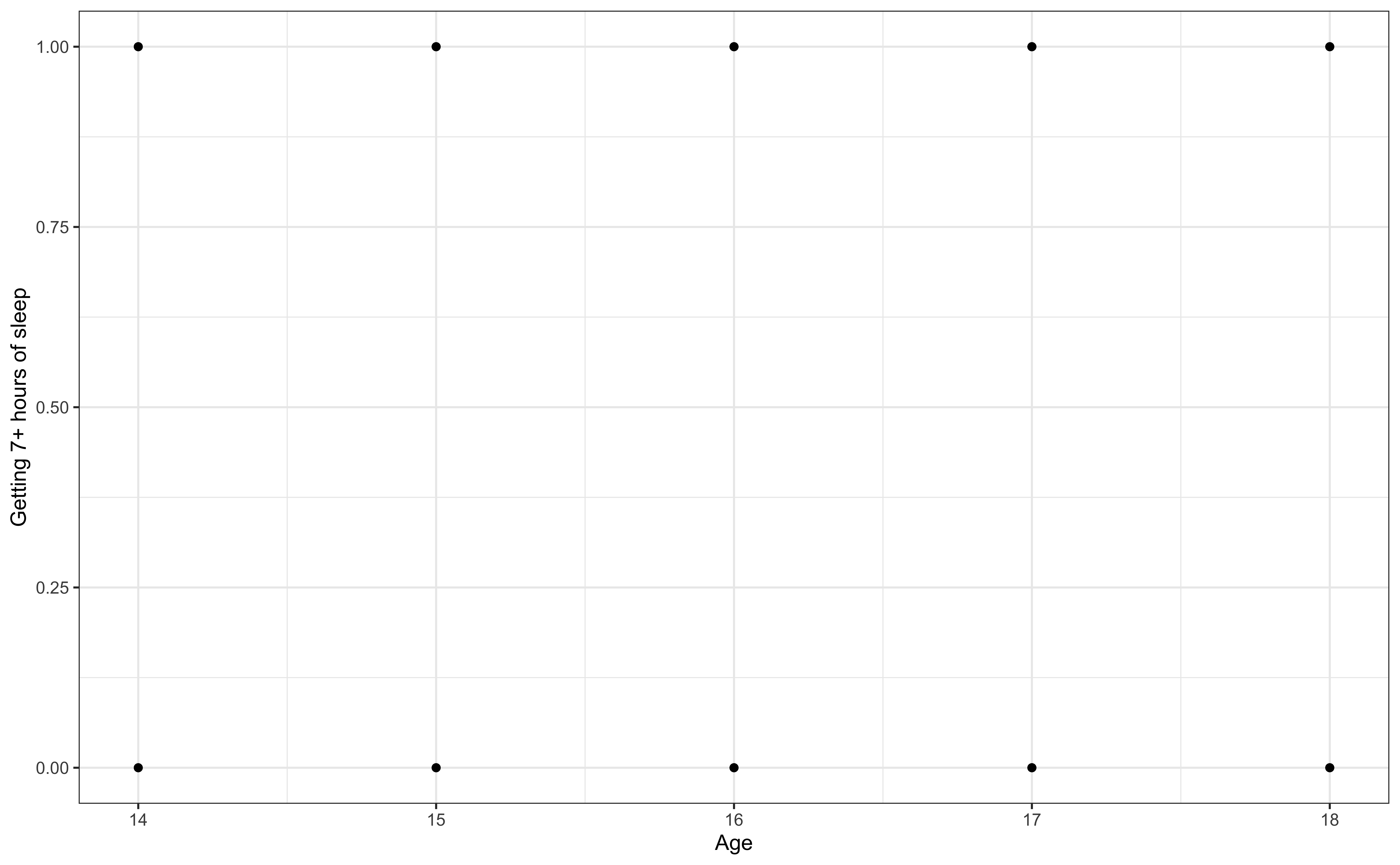
Let’s fit a linear regression model
Outcome: \(Y\) = 1: yes, 0: no
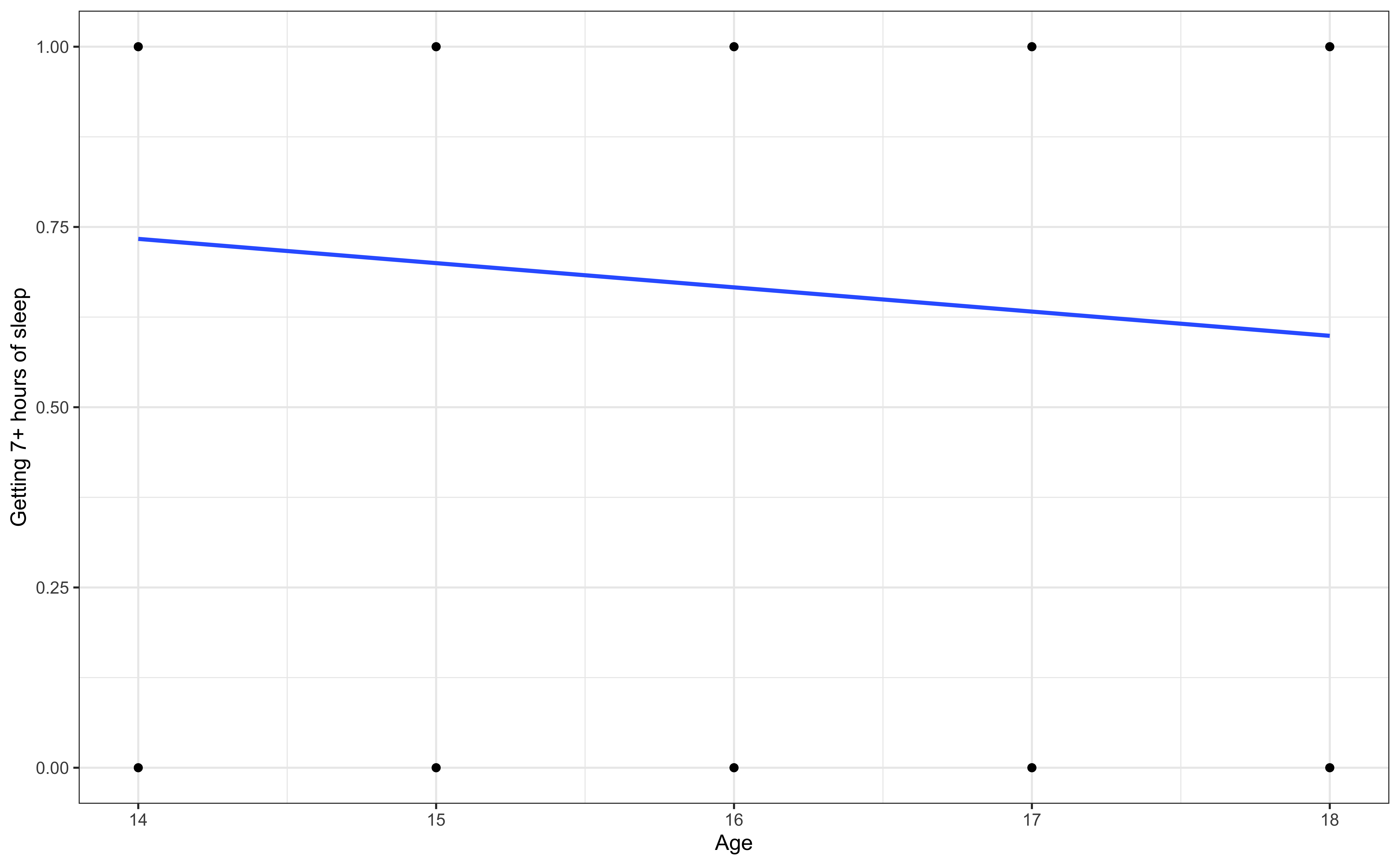
Let’s use proportions
Outcome: Probability of getting 7+ hours of sleep
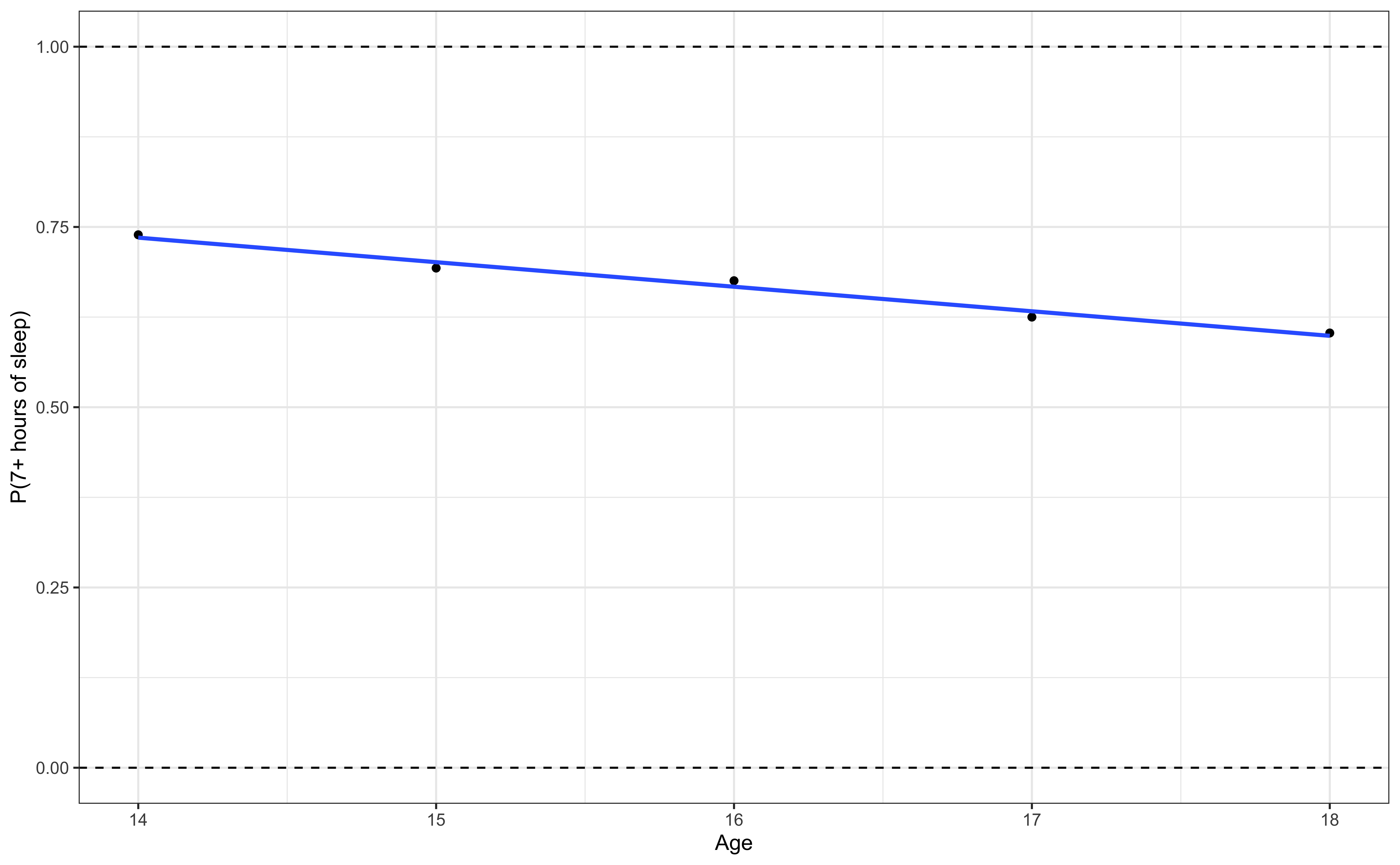
What happens if we zoom out?
Outcome: Probability of getting 7+ hours of sleep
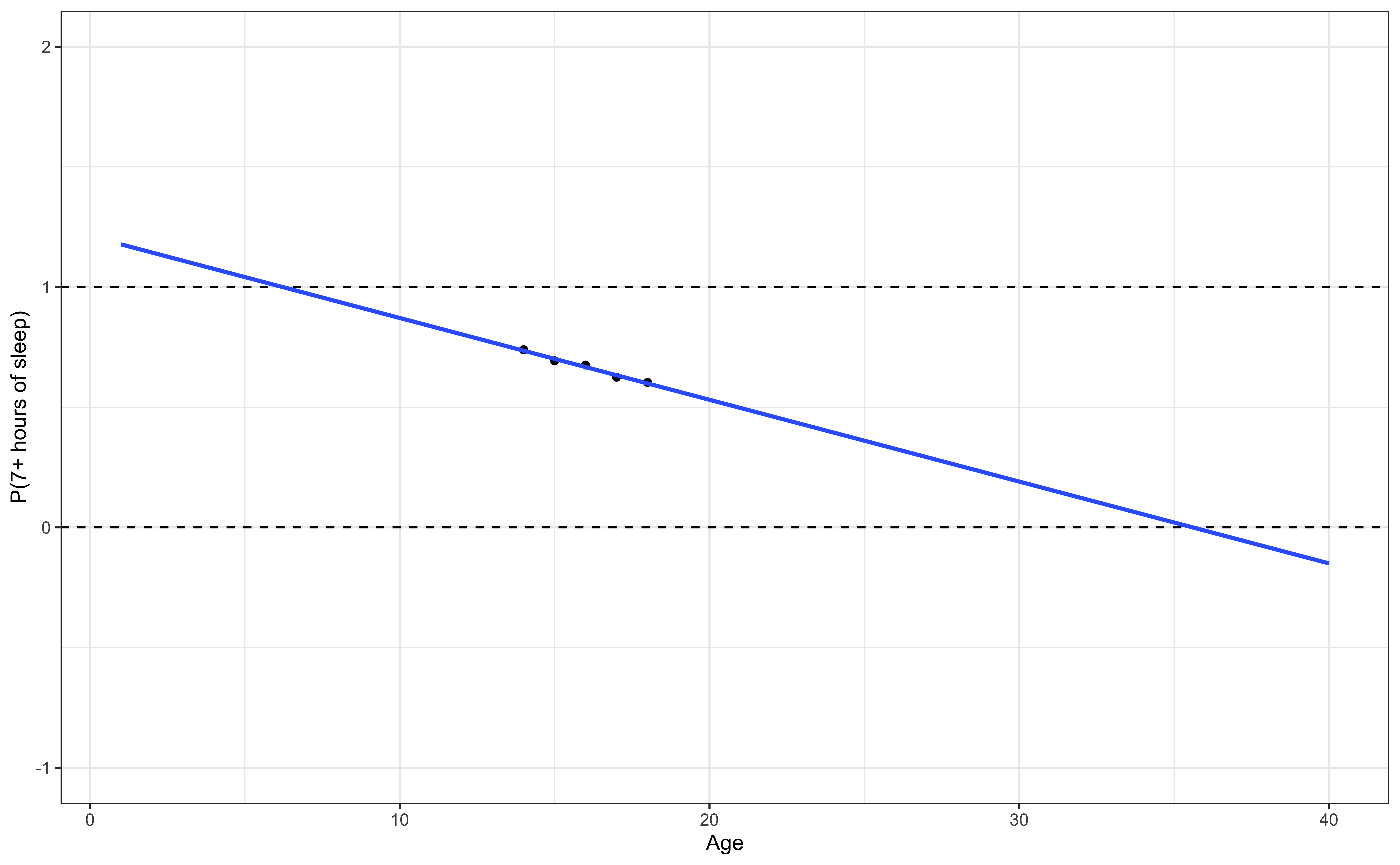
🛑 This model produces predictions outside of 0 and 1.
Let’s try another model
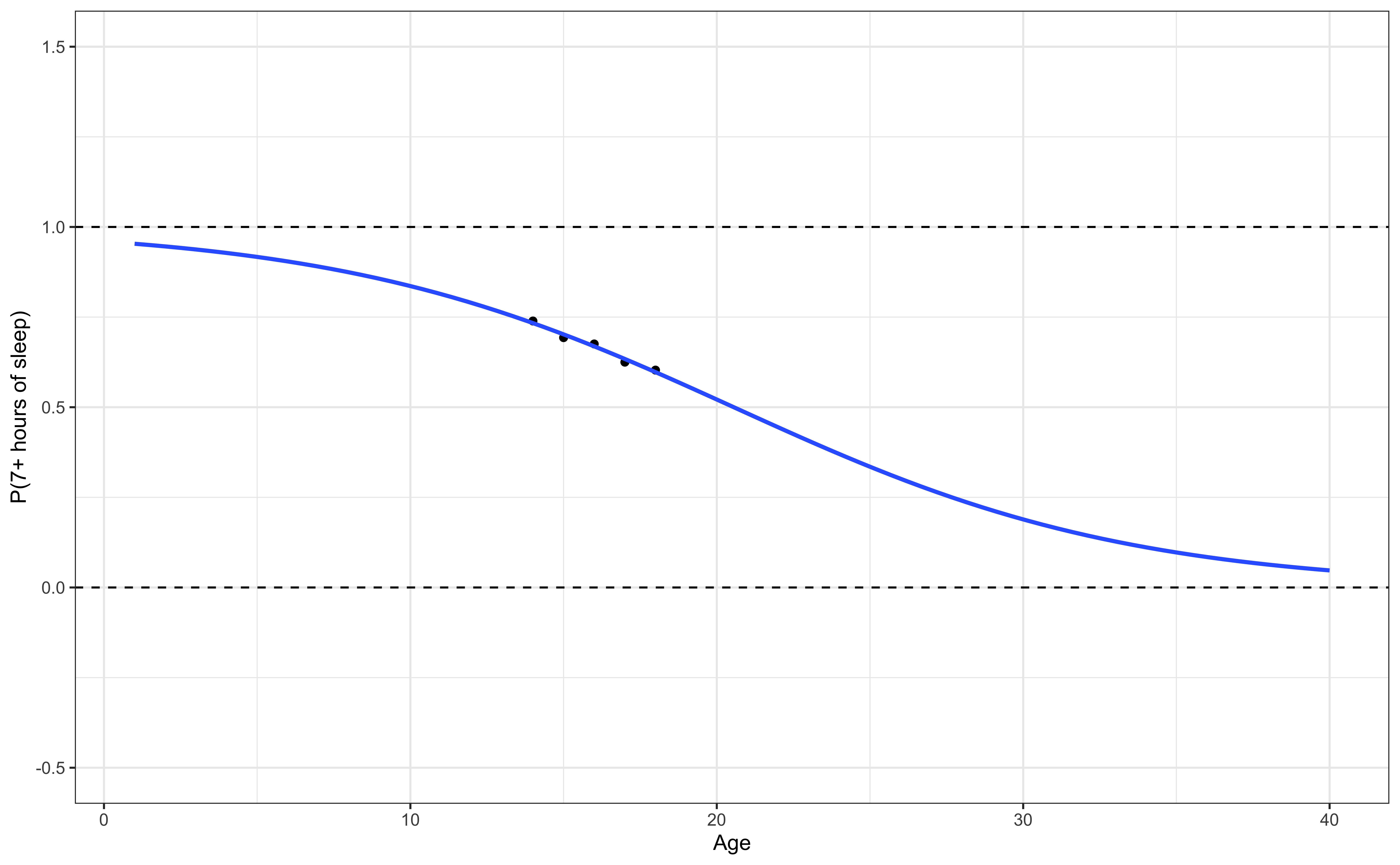
✅ This model (called a logistic regression model) only produces predictions between 0 and 1.
The code
Different types of models
| Method | Outcome | Model |
|---|---|---|
| Linear regression | Quantitative | \(y_i = \beta_0 + \beta_1~ x_i\) |
| Linear regression (transform Y) | Quantitative | \(\log(y_i) = \beta_0 + \beta_1~ x_i\) |
| Logistic regression | Binary | \(\log\big(\frac{\pi_i}{1-\pi_i}\big) = \beta_0 + \beta_1 ~ x_i\) |
Linear vs. logistic regression
State whether a linear regression model or logistic regression model is more appropriate for each scenario.
Use age and education to predict if a randomly selected person will vote in the next election.
Use budget and run time (in minutes) to predict a movie’s total revenue.
Use age and sex to calculate the probability a randomly selected adult will visit Duke Health in the next year.
Probabilities and odds
Binary response variable
- \(Y = 1: \text{ yes}, 0: \text{ no}\)
- \(\pi\): probability that \(Y=1\), i.e., \(P(Y = 1)\)
- \(\frac{\pi}{1-\pi}\): odds that \(Y = 1\)
- \(\log\big(\frac{\pi}{1-\pi}\big)\): log odds
- Go from \(\pi\) to \(\log\big(\frac{\pi}{1-\pi}\big)\) using the logit transformation
Odds
Suppose there is a 70% chance it will rain tomorrow
- Probability it will rain is \(\mathbf{p = 0.7}\)
- Probability it won’t rain is \(\mathbf{1 - p = 0.3}\)
- Odds it will rain are 7 to 3, 7:3, \(\mathbf{\frac{0.7}{0.3} \approx 2.33}\)
Are teenagers getting enough sleep?
# A tibble: 2 × 3
  Sleep7     n     p
   <int> <int> <dbl>
1      0   150 0.336
2      1   296 0.664
\(P(\text{7+ hours of sleep}) = P(Y = 1) = p = 0.664\)
\(P(\text{< 7 hours of sleep}) = P(Y = 0) = 1 - p = 0.336\)
\(\text{odds of 7+ hours of sleep} = \frac{0.664}{0.336} = 1.976\)
From odds to probabilities
odds
\[\omega = \frac{\pi}{1-\pi}\]
probability
\[\pi = \frac{\omega}{1 + \omega}\]
Odds ratios
Risk of coronary heart disease
This data set is from an ongoing cardiovascular study on residents of the town of Framingham, Massachusetts. We want to examine the relationship between various health characteristics and the risk of having heart disease. These notes focus on the following variables:
high_risk:- 1: High risk of having heart disease in next 10 years
- 0: Not high risk of having heart disease in next 10 year
education: 1 = Some High School, 2 = High School or GED, 3 = Some College or Vocational School, 4 = College
High risk vs. education
| Education | High risk | Not high risk |
|---|---|---|
| Some high school | 323 | 1397 |
| High school or GED | 147 | 1106 |
| Some college or vocational school | 88 | 601 |
| College | 70 | 403 |
Compare the odds for two groups
| Education | High risk | Not high risk |
|---|---|---|
| Some high school | 323 | 1397 |
| High school or GED | 147 | 1106 |
| Some college or vocational school | 88 | 601 |
| College | 70 | 403 |
We want to compare the risk of heart disease for those with a High School diploma/GED and those with a college degree.
We’ll use the odds to compare the two groups
\[ \text{odds} = \frac{P(\text{success})}{P(\text{failure})} = \frac{\text{# of successes}}{\text{# of failures}} \]
Compare the odds for two groups
| Education | High risk | Not high risk |
|---|---|---|
| Some high school | 323 | 1397 |
| High school or GED | 147 | 1106 |
| Some college or vocational school | 88 | 601 |
| College | 70 | 403 |
Odds of being high risk for the High school or GED group: \(\frac{147}{1106} = 0.133\)
Odds of being high risk for the College group: \(\frac{70}{403} = 0.174\)
Based on this, we see those with a college degree had higher odds of being high risk for heart disease than those with a high school diploma or GED.
Odds ratio (OR)
| Education | High risk | Not high risk |
|---|---|---|
| Some high school | 323 | 1397 |
| High school or GED | 147 | 1106 |
| Some college or vocational school | 88 | 601 |
| College | 70 | 403 |
Let’s summarize the relationship between the two groups. To do so, we’ll use the odds ratio (OR).
\[ OR = \frac{\text{odds}_1}{\text{odds}_2} = \frac{\omega_1}{\omega_2} \]
OR: College vs. High school or GED
| Education | High risk | Not high risk |
|---|---|---|
| Some high school | 323 | 1397 |
| High school or GED | 147 | 1106 |
| Some college or vocational school | 88 | 601 |
| College | 70 | 403 |
\[OR = \frac{\text{odds}_{College}}{\text{odds}_{HS}} = \frac{0.174}{0.133} = \mathbf{1.308}\]
The odds of being high risk for heart disease are 1.30 times higher for those with a college degree than those with a high school diploma or GED.
OR: College vs. Some high school
| Education | High risk | Not high risk |
|---|---|---|
| Some high school | 323 | 1397 |
| High school or GED | 147 | 1106 |
| Some college or vocational school | 88 | 601 |
| College | 70 | 403 |
\[OR = \frac{\text{odds}_{College}}{\text{odds}_{Some HS}} = \frac{70/403}{323/1397} = 0.751\]
The odds of being high risk for having heart disease for those with a college degree are 0.751 times the odds of being high risk for heart disease for those with some high school.
More natural interpretation
It’s more natural to interpret the odds ratio with a statement with the odds ratio greater than 1.
The odds of being high risk for heart disease are 1.33 times higher for those with some high school than those with a college degree.
Making the table 1
First, rename the levels of the categorical variables:
heart_disease <- heart_disease |>
  mutate(
    high_risk_names = if_else(high_risk == "1", "High risk", "Not high risk"),
    education_names = case_when(
      education == "1" ~ "Some high school",
      education == "2" ~ "High school or GED",
      education == "3" ~ "Some college or vocational school",
      education == "4" ~ "College"
    ),
    education_names = fct_relevel(education_names, "Some high school", "High school or GED", "Some college or vocational school", "College")
  )
Making the table 2
Then, make the table:
Deeper look into the code
# A tibble: 8 × 3
education_names high_risk_names n
<fct> <chr> <int>
1 Some high school High risk 323
2 Some high school Not high risk 1397
3 High school or GED High risk 147
4 High school or GED Not high risk 1106
5 Some college or vocational school High risk 88
6 Some college or vocational school Not high risk 601
7 College High risk 70
8 College Not high risk 403Deeper look into the code
heart_disease |>
count(education_names, high_risk_names) |>
pivot_wider(names_from = high_risk_names, values_from = n)# A tibble: 4 × 3
education_names `High risk` `Not high risk`
<fct> <int> <int>
1 Some high school 323 1397
2 High school or GED 147 1106
3 Some college or vocational school 88 601
4 College 70 403Deeper look into the code
Deeper look into the code
heart_disease |>
  count(education_names, high_risk_names) |>
  pivot_wider(names_from = high_risk_names, values_from = n) |>
kable(col.names = c("Education", "High risk", "Not high risk"))| Education | High risk | Not high risk |
|---|---|---|
| Some high school | 323 | 1397 |
| High school or GED | 147 | 1106 |
| Some college or vocational school | 88 | 601 |
| College | 70 | 403 |
Application exercise
If your group is selected, click here to add your response to the Google Slide.
Recap
Introduced logistic regression for binary response variable
Showed the relationship between odds and probabilities
Introduced odds ratios and their connection to logistic model
