Logistic Regression: Inference

Prof. Maria Tackett

Nov 14, 2024

Announcements

Project: Draft report due + peer review in December 2 lab
Statistics experience due Tuesday, November 26
HW 04 released later today. Due Thursday, November 21

Topics

Test of significance for overall logistic regression model
Test of significance for a subset of model coefficients
Test of significance for a single coefficient

Computational setup

library(tidyverse)
library(tidymodels)
library(pROC)      
library(knitr)
library(kableExtra)

# set default theme in ggplot2
ggplot2::theme_set(ggplot2::theme_bw())

Risk of coronary heart disease

This data set is from an ongoing cardiovascular study on residents of the town of Framingham, Massachusetts. We want to examine the relationship between various health characteristics and the risk of having heart disease.

high_risk:
- 1: High risk of having heart disease in next 10 years
- 0: Not high risk of having heart disease in next 10 years
age: Age at exam time (in years)
totChol: Total cholesterol (in mg/dL)
currentSmoker: 0 = nonsmoker, 1 = smoker
education: 1 = Some High School, 2 = High School or GED, 3 = Some College or Vocational School, 4 = College

Modeling risk of coronary heart disease

Using age, totChol, currentSmoker

heart_disease_fit <- glm(high_risk ~ age + totChol + currentSmoker, 
              data = heart_disease, family = "binomial")

tidy(heart_disease_fit, conf.int = TRUE) |> 
  kable(digits = 3)

term	estimate	std.error	statistic	p.value	conf.low	conf.high
(Intercept)	-6.673	0.378	-17.647	0.000	-7.423	-5.940
age	0.082	0.006	14.344	0.000	0.071	0.094
totChol	0.002	0.001	1.940	0.052	0.000	0.004
currentSmoker1	0.443	0.094	4.733	0.000	0.260	0.627

Test for overall significance

Likelihood ratio test

Similar to linear regression, we can test the overall significance for a logistic regression model, i.e., whether there is at least one non-zero coefficient in the model

\[ \begin{aligned} &H_0: \beta_1 = \dots = \beta_p = 0 \\ &H_a: \beta_j \neq 0 \text{ for at least one } j \end{aligned} \]

The likelihood ratio test compares the fit of a model with no predictors to the current model.

Likelihood ratio test statistic

Let \(L_0\) and \(L_a\) be the likelihood functions of the model under \(H_0\) and \(H_a\), respectively. The likelihood ratio test statistic is

\[ G = -2[\log L_0 - \log L_a] = -2\sum_{i=1}^n \Big[ y_i \log \Big(\frac{\hat{\pi}^0}{\hat{\pi}^a_i}\Big) + (1 - y_i)\log \Big(\frac{1-\hat{\pi}^0}{1-\hat{\pi}^a_i}\Big)\Big] \]

where \(\hat{\pi}^0\) is the predicted probability under \(H_0\) and \(\hat{\pi}_i^a = \frac{\exp \{x_i^T\boldsymbol{\beta}\}}{1 + \exp \{x_i^T\boldsymbol{\beta}\}}\) is the predicted probability under \(H_a\) ¹

Likelihood ratio test statistic

\[ G = -2\sum_{i=1}^n \Big[ y_i \log \Big(\frac{\hat{\pi}^0}{\hat{\pi}^a_i}\Big) + (1 - y_i)\log \Big(\frac{1-\hat{\pi}^0}{1-\hat{\pi}^a_i}\Big)\Big] \]

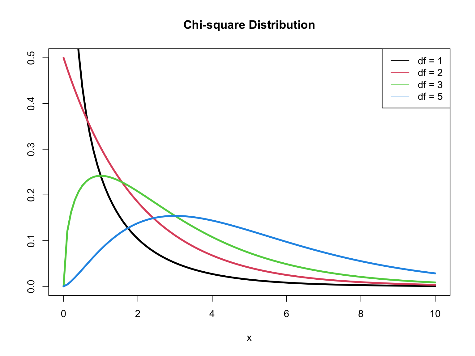
When \(n\) is large, \(G \sim \chi^2_p\), ( \(G\) follows a Chi-square distribution with \(p\) degrees of freedom)
The p-value is calculated as \(\text{p-value} = P(\chi^2 > G)\)
Large values of \(G\) (small p-values) indicate at least one \(\beta_j\) is non-zero

\(\chi^2\) distribution

Heart disease model: likelihood ratio test

\[ \begin{aligned} &H_0: \beta_{age} = \beta_{totChol} = \beta_{currentSmoker} = 0 \\ &H_a: \beta_j \neq 0 \text{ for at least one }j \end{aligned}\]

Fit the null model

(we’ve already fit the alternative model)

null_model <- glm(high_risk ~ 1, data = heart_disease, family = "binomial")

tidy(null_model) |>
  kable()

term	estimate	std.error	statistic	p.value
(Intercept)	-1.72294	0.0436342	-39.486	0

Heart disease model: likelihood ratio test

Calculate the log-likelihood for the null and alternative models

(L_0 <- glance(null_model)$logLik)

[1] -1737.735

(L_a <- glance(heart_disease_fit)$logLik)

[1] -1612.406

Calculate the likelihood ratio test statistic

(G <- -2 * (L_0 - L_a))

[1] 250.6572

Heart disease model: likelihood ratio test

Calculate the p-value

(p_value <- pchisq(G, df = 3, lower.tail = FALSE))

[1] 4.717158e-54

Conclusion

The p-value is small, so we reject \(H_0\). The data provide evidence of at least one non-zero model coefficient in the model.

Test a subset of coefficients

Testing a subset of coefficients

Suppose there are two models:
- Reduced Model: includes predictors \(x_1, \ldots, x_q\)
- Full Model: includes predictors \(x_1, \ldots, x_q, x_{q+1}, \ldots, x_p\)
We can use the likelihood ratios to see if any of the new predictors are useful

\[ \begin{aligned} &H_0: \beta_{q+1} = \dots = \beta_p = 0\\ &H_a: \beta_j \neq 0 \text{ for at least one }j \end{aligned} \]

This is called a drop-in-deviance test (also known as nested likelihood ratio test)

Deviance

The deviance is a measure of the degree to which the predicted values are different from the observed values (compares the current model to a “saturated” model)

In logistic regression,

\[ D = -2 \log L \]

\(D \sim \chi^2_{n - p - 1}\) ( \(D\) follows a Chi-square distribution with \(n - p - 1\) degrees of freedom)

Note: \(n - p - 1\) a the degrees of freedom associated with the error in the model (like residuals)

Drop-in-deviance test

\[ \begin{aligned} &H_0: \beta_{q+1} = \dots = \beta_p = 0\\ &H_a: \beta_j \neq 0 \text{ for at least one }j \end{aligned} \]

The test statistic is

\[ \begin{aligned} G = D_{reduced} - D_{full} &= -2\log L_{reduced} - (-2 \log L_{full}) \\ &= -2(\log L_{reduced} - \log L_{full}) \end{aligned} \]

The p-value is calculated using a \(\chi_{\Delta df}^2\) distribution, where \(\Delta df\) is the number of parameters being tested (the difference in number of parameters between the full and reduced model).

Heart disease model: drop-in-deviance test

Should we add education to the model?

Reduced model: age, totChol, currentSmoker
Full model: age, totChol, currentSmoker , education

\[ \begin{aligned} &H_0: \beta_{ed1} = \beta_{ed2} = \beta_{ed3} = 0 \\ &H_a: \beta_j \neq 0 \text{ for at least one }j \end{aligned} \]

Heart disease model: drop-in-deviance test

reduced_model <- glm(high_risk ~ age + totChol + currentSmoker, 
              data = heart_disease, family = "binomial")

full_model <- glm(high_risk ~ age + totChol + currentSmoker + education, 
              data = heart_disease, family = "binomial")

Calculate deviances

(deviance_reduced <- -2 * glance(reduced_model)$logLik)

[1] 3224.812

(deviance_full <- -2 * glance(full_model)$logLik)

[1] 3217.6

Calculate test statistic

(G <- deviance_reduced - deviance_full)

[1] 7.212113

Heart disease model: drop-in-deviance test

Calculate p-value

pchisq(G, df = 3, lower.tail = FALSE)

[1] 0.06543567

What is your conclusion? Would you include education in the model that already has age, totChol, currentSmoker?

Drop-in-deviance test in R

Conduct the drop-in-deviance test using the anova() function in R with option test = "Chisq"

anova(reduced_model, full_model, test = "Chisq") |> 
  tidy() |> 
  kable(digits = 3)

term	df.residual	residual.deviance	df	deviance	p.value
high_risk ~ age + totChol + currentSmoker	4082	3224.812	NA	NA	NA
high_risk ~ age + totChol + currentSmoker + education	4079	3217.600	3	7.212	0.065

AIC and BIC

Similar to linear regression, we can use AIC and BIC to compare models.

\[ \begin{aligned} &AIC = -2 \log L + 2(p+1) \\ &BIC = -2 \log L + \log(n)(p + 1) \end{aligned} \]

You want to select the model that minimizes AIC / BIC

Compare models using AIC

AIC for reduced model (age, totChol, currentSmoker)

glance(reduced_model)$AIC

[1] 3232.812

AIC for full model (age, totChol, currentSmoker, education)

glance(full_model)$AIC

[1] 3231.6

Compare models using BIC

BIC for reduced model (age, totChol, currentSmoker)

glance(reduced_model)$BIC

[1] 3258.074

BIC for full model (age, totChol, currentSmoker, education)

glance(full_model)$BIC

[1] 3275.807

Test for a single coefficient

Distribution of \(\hat{\boldsymbol{\beta}}\)

When \(n\) is large, \(\hat{\boldsymbol{\beta}}\), the estimated coefficients of the logistic regression model, is approximately normal.

How do we know the distribution of \(\hat{\boldsymbol{\beta}}\) is normal for large \(n\)?

Distribution of \(\hat{\boldsymbol{\beta}}\)

The expected value of \(\hat{\boldsymbol{\beta}}\) is the true parameter, \(\boldsymbol{\beta}\), i.e., \(E(\hat{\boldsymbol{\beta}}) = \boldsymbol{\beta}\)

\(Var(\hat{\boldsymbol{\beta}})\), the matrix of variances and covariances between estimators, is found by taking the second partial derivatives of the log-likelihood function (Hessian matrix)

\[ Var(\hat{\boldsymbol{\beta}}) = (\mathbf{X}^T\mathbf{V}\mathbf{X})^{-1} \]

where \(\mathbf{V}\) is a \(n\times n\) diagonal matrix such that \(V_{ii}\) is the estimated variance for the \(i^{th}\) observation

Test for a single coefficient

Hypotheses: \(H_0: \beta_j = 0 \hspace{2mm} \text{ vs } \hspace{2mm} H_a: \beta_j \neq 0\), given the other variables in the model

(Wald) Test Statistic: \[z = \frac{\hat{\beta}_j - 0}{SE(\hat{\beta}_j)}\]

where \(SE(\hat{\beta}_j)\) is the square root of the \(j^{th}\) diagonal element of \(Var(\hat{\boldsymbol{\beta}})\)

P-value: \(P(|Z| > |z|)\), where \(Z \sim N(0, 1)\), the Standard Normal distribution

Confidence interval for \(\beta_j\)

We can calculate the C% confidence interval for \(\beta_j\) as the following:

\[ \Large{\hat{\beta}_j \pm z^* SE(\hat{\beta}_j)} \]

where \(z^*\) is calculated from the \(N(0,1)\) distribution

Note

This is an interval for the change in the log-odds for every one unit increase in \(x_j\)

Interpretation in terms of the odds

The change in odds for every one unit increase in \(x_j\).

\[ \Large{\exp\{\hat{\beta}_j \pm z^* SE(\hat{\beta}_j)\}} \]

Interpretation: We are \(C\%\) confident that for every one unit increase in \(x_j\), the odds multiply by a factor of \(\exp\{\hat{\beta}_j - z^* SE(\hat{\beta}_j)\}\) to \(\exp\{\hat{\beta}_j + z^* SE(\hat{\beta}_j)\}\), holding all else constant.

Coefficient for `age`

term	estimate	std.error	statistic	p.value	conf.low	conf.high
(Intercept)	-6.673	0.378	-17.647	0.000	-7.423	-5.940
age	0.082	0.006	14.344	0.000	0.071	0.094
totChol	0.002	0.001	1.940	0.052	0.000	0.004
currentSmoker1	0.443	0.094	4.733	0.000	0.260	0.627

Hypotheses:

\[ H_0: \beta_{age} = 0 \hspace{2mm} \text{ vs } \hspace{2mm} H_a: \beta_{age} \neq 0 \], given total cholesterol and smoking status are in the model.

Coefficient for `age`

term	estimate	std.error	statistic	p.value	conf.low	conf.high
(Intercept)	-6.673	0.378	-17.647	0.000	-7.423	-5.940
age	0.082	0.006	14.344	0.000	0.071	0.094
totChol	0.002	0.001	1.940	0.052	0.000	0.004
currentSmoker1	0.443	0.094	4.733	0.000	0.260	0.627

Test statistic:

\[z = \frac{ 0.0825 - 0}{0.00575} = 14.34 \]

Coefficient for `age`

term	estimate	std.error	statistic	p.value	conf.low	conf.high
(Intercept)	-6.673	0.378	-17.647	0.000	-7.423	-5.940
age	0.082	0.006	14.344	0.000	0.071	0.094
totChol	0.002	0.001	1.940	0.052	0.000	0.004
currentSmoker1	0.443	0.094	4.733	0.000	0.260	0.627

P-value:

\[P(|Z| > |14.34|) \approx 0 \]

2 * pnorm(14.34,lower.tail = FALSE)

[1] 1.230554e-46

Coefficient for `age`

term	estimate	std.error	statistic	p.value	conf.low	conf.high
(Intercept)	-6.673	0.378	-17.647	0.000	-7.423	-5.940
age	0.082	0.006	14.344	0.000	0.071	0.094
totChol	0.002	0.001	1.940	0.052	0.000	0.004
currentSmoker1	0.443	0.094	4.733	0.000	0.260	0.627

Conclusion:

The p-value is very small, so we reject \(H_0\). The data provide sufficient evidence that age is a statistically significant predictor of whether someone is high risk of having heart disease, after accounting for total cholesterol and smoking status.

CI for `age`

term	estimate	std.error	statistic	p.value	conf.low	conf.high
(Intercept)	-6.673	0.378	-17.647	0.000	-7.423	-5.940
age	0.082	0.006	14.344	0.000	0.071	0.094
totChol	0.002	0.001	1.940	0.052	0.000	0.004
currentSmoker1	0.443	0.094	4.733	0.000	0.260	0.627

Interpret the 95% confidence interval for age in terms of the odds of being high risk for heart disease.

Overview of testing coefficients

Test a single coefficient

Likelihood ratio test
Drop-in-deviance test
Wald hypothesis test and confidence interval

Test a subset of coefficients

Likelihood ratio test
Drop-in-deviance test

Can use AIC and BIC to compare models in both scenarios

References

Wilks, SS. 1935. “The Likelihood Test of Independence in Contingency Tables.” The Annals of Mathematical Statistics 6 (4): 190–96.

Logistic Regression: Inference

Announcements

Topics

Computational setup

Risk of coronary heart disease

Modeling risk of coronary heart disease

Test for overall significance

Likelihood ratio test

Likelihood ratio test statistic

Likelihood ratio test statistic

\(\chi^2\) distribution

Heart disease model: likelihood ratio test

Heart disease model: likelihood ratio test

Heart disease model: likelihood ratio test

Test a subset of coefficients

Testing a subset of coefficients

Deviance

Drop-in-deviance test

Heart disease model: drop-in-deviance test

Heart disease model: drop-in-deviance test

Heart disease model: drop-in-deviance test

Drop-in-deviance test in R

AIC and BIC

Compare models using AIC

Compare models using BIC

Test for a single coefficient

Distribution of \(\hat{\boldsymbol{\beta}}\)

Distribution of \(\hat{\boldsymbol{\beta}}\)

Test for a single coefficient

Confidence interval for \(\beta_j\)

Interpretation in terms of the odds

Coefficient for age

Coefficient for age

Coefficient for age

Coefficient for age

CI for age

Overview of testing coefficients

References

Coefficient for `age`

Coefficient for `age`

Coefficient for `age`

Coefficient for `age`

CI for `age`